Iniciar o QAOA com o Qiskit addon Optimization Mapper

Estimativa de uso: 9 minutos em um Heron r3 (NOTA: Isso é apenas uma estimativa. Seu tempo de execução pode variar.)

Resultados de aprendizagem

• Como mapear um problema de max-cut para uma formulação de Otimização Binária Quadrática Irrestrita (QUBO) quântica usando qiskit-addon-opt-mapper

• Como implementar e executar o QAOA padrão em um simulador

• Como aplicar o WS-QAOA calculando a relaxação do programa quadrático (QP) e construindo o circuito de warm-start

• Como comparar a convergência de energia e a qualidade da solução entre o QAOA padrão e o WS-QAOA

Pré-requisitos

• Tutorial de QAOA

• Tutorial avançado de QAOA

Histórico

O Quantum Approximate Optimization Algorithm (QAOA) é um algoritmo híbrido quântico-clássico projetado para resolver problemas de otimização combinatória, como max-cut e formulações QUBO gerais. Para uma introdução fundamental ao QAOA no Qiskit, veja o tutorial de QAOA; para técnicas mais avançadas de construção de circuitos, veja o tutorial avançado de QAOA.

No QAOA padrão:

• O estado inicial é a superposição uniforme $|+\rangle^{\otimes n}$.
• Os parâmetros variacionais são inicializados aleatoriamente.
• Um otimizador clássico busca parâmetros que minimizem a função de custo.

No entanto, para tamanhos práticos de problema e hardware quântico ruidoso, a inicialização aleatória pode levar a uma convergência lenta, mínimos locais ruins e maior custo de otimização.

Warm-start QAOA (WS-QAOA) melhora isso incorporando percepções de otimização clássica diretamente no circuito quântico. Este tutorial segue os métodos introduzidos por Egger, Mareček e Woerner em Warm-starting quantum optimization. A ideia principal é:

1. Resolver uma relaxação contínua do problema binário original (um programa quadrático sobre $[0,1]^n$ em vez de $\{0,1\}^n$).

2. Codificar a solução relaxada $c^*_i \in [0,1]$ em um estado inicial personalizado usando ângulos de rotação $Y$ $\theta_i = 2\arcsin(\sqrt{c^*_i})$, de modo que o qubit $i$ comece em um estado cuja probabilidade de medir $|1\rangle$ seja $c^*_i$.

3. Substituir o mixer $X$ padrão por um mixer personalizado cujo estado fundamental é o estado inicial de warm-start, garantindo que o algoritmo comece perto da solução clássica e possa explorar a vizinhança.

Um parâmetro de regularização $\varepsilon \in [0, 0.5]$ afasta $c^*_i$ de 0 e 1 para evitar problemas de alcançabilidade; qubits inicializados em $|0\rangle$ ou $|1\rangle$ não podem ser movidos pelo Hamiltoniano de custo. Em $\varepsilon = 0.5$, o WS-QAOA se reduz exatamente ao QAOA padrão.

A modelagem do problema usa o pacote qiskit-addon-opt-mapper, cuja classe de aplicação Maxcut constrói o QUBO diretamente a partir de um grafo, e cujos conversores e tradutores mapeiam o problema resultante para Hamiltonianos quânticos.

Requisitos

Antes de iniciar este tutorial, certifique-se de ter instalado o seguinte:

• Qiskit SDK v2.0 ou posterior, com suporte a visualização

• Qiskit Runtime v0.43 ou posterior (pip install qiskit-ibm-runtime)

• Qiskit addon Optimization Mapper (pip install qiskit-addon-opt-mapper)

• SciPy (pip install scipy)

• NetworkX (pip install networkx)

Configuração

Importe todas as bibliotecas necessárias e defina as funções auxiliares usadas ao longo deste tutorial.

# Added by doQumentation — required packages for this notebook
!pip install -q matplotlib networkx numpy qiskit qiskit-addon-opt-mapper qiskit-ibm-runtime scipy

import numpy as np
import matplotlib.pyplot as plt
import networkx as nx
from scipy.optimize import minimize

from qiskit.circuit import QuantumCircuit, ParameterVector
from qiskit.circuit.library import qaoa_ansatz
from qiskit.quantum_info import Statevector
from qiskit.primitives import StatevectorEstimator, StatevectorSampler
from qiskit.transpiler.preset_passmanagers import generate_preset_pass_manager
from qiskit_ibm_runtime import (
    QiskitRuntimeService,
    Session,
    EstimatorOptions,
    EstimatorV2 as Estimator,
    SamplerV2 as Sampler,
)

from qiskit_addon_opt_mapper.applications import Maxcut
from qiskit_addon_opt_mapper.converters import OptimizationProblemToQubo
from qiskit_addon_opt_mapper.translators import to_ising

Exemplo de simulador em pequena escala

Usamos um pequeno problema de max-cut em um grafo ponderado como nosso exemplo de referência. O max-cut pergunta: dado um grafo $G=(V,E)$ com pesos de aresta $w_{ij}$, encontre uma partição dos vértices em dois conjuntos $S$ e $\bar{S}$ que maximize o peso total das arestas que cruzam o corte.

Como um problema de minimização QUBO, o max-cut pode ser escrito como: $\min_{x \in \{0,1\}^n} -\sum_{(i,j) \in E} w_{ij}(x_i + x_j - 2x_i x_j)$

Trabalhamos com um grafo de quatro nós para tornar o problema tratável em um simulador.

Passo 1: Mapear entradas clássicas para um problema quântico

Definimos o problema de max-cut usando a classe de aplicação Maxcut de qiskit-addon-opt-mapper, que constrói a formulação QUBO diretamente a partir de um grafo. Em seguida, o convertemos para um QUBO e o traduzimos para um Hamiltoniano de Ising (SparsePauliOp) adequado para o QAOA. Também resolvemos a relaxação contínua do QUBO — substituindo a restrição binária $x_i \in \{0,1\}$ por $x_i \in [0,1]$ — para obter o ponto inicial de warm-start $c^*$.

# Define a 4-node weighted graph for the max-cut problem
n_nodes = 4
edges = [(0, 1, 1.0), (0, 2, 1.0), (1, 2, 1.0), (1, 3, 1.0), (2, 3, 1.0)]

G = nx.Graph()
G.add_nodes_from(range(n_nodes))
G.add_weighted_edges_from(edges)

pos = nx.spring_layout(G, seed=42)
edge_labels = {(u, v): d["weight"] for u, v, d in G.edges(data=True)}

fig, ax = plt.subplots(figsize=(4, 3))
nx.draw(G, pos, with_labels=True, node_color="lightblue", ax=ax)
nx.draw_networkx_edge_labels(G, pos, edge_labels=edge_labels, ax=ax)
ax.set_title("Max-Cut graph")
plt.tight_layout()
plt.show()

O grafo tem cinco arestas. O max-cut ótimo particiona os nós em $S = \{0, 3\}$ e $\bar{S} = \{1, 2\}$ (ou seu complemento), rompendo quatro das cinco arestas para um valor de corte de 4.

# Build the max-cut problem directly from the NetworkX graph using the
# Maxcut application class. Internally it constructs the QUBO
#   minimize  -sum_{(i,j) in E} w_ij * (x_i + x_j - 2*x_i*x_j)
# (each edge contributes -w to the linear terms and +2w to the quadratic
# term), so we get the same OptimizationProblem without the boilerplate.
maxcut = Maxcut(G)
prob = maxcut.to_optimization_problem()
print(prob.prettyprint())

Problem name: Max-cut

Maximize
  -2*x_0*x_1 - 2*x_0*x_2 - 2*x_1*x_2 - 2*x_1*x_3 - 2*x_2*x_3 + 2*x_0 + 3*x_1
  + 3*x_2 + 2*x_3

Subject to
  No constraints

  Binary variables (4)
    x_0 x_1 x_2 x_3

A classe Maxcut encapsula a construção do QUBO para que não precisemos expandir manualmente o objetivo do max-cut. O objetivo impresso mostra o coeficiente linear de cada variável (o quanto ela individualmente contribui para o corte) e o coeficiente quadrático de cada termo cruzado (a penalidade por colocar dois nós adjacentes no mesmo lado). O OptimizationProblem subjacente retornado por to_optimization_problem() suporta variáveis binárias, inteiras, contínuas e de spin, e é o mesmo objeto esperado pelos conversores e tradutores usados no próximo passo.

# Convert the OptimizationProblem to a QUBO, then translate to an Ising Hamiltonian
#
# The substitution x_i = (1 - z_i)/2  maps binary variables to spin operators,
# yielding a Hamiltonian H_C = sum_i h_i Z_i + sum_{i<j} J_ij Z_i Z_j + constant.
# QAOA minimizes <H_C> to find the ground state, which encodes the optimal cut.
converter = OptimizationProblemToQubo()
qubo = converter.convert(prob)

cost_operator, offset = to_ising(qubo)
n_qubits = cost_operator.num_qubits

print(f"Cost Hamiltonian H_C ({n_qubits} qubits):")
print(cost_operator)
print(f"\nOffset (constant shift): {offset}")
print("  QUBO value = Ising energy + offset")

Cost Hamiltonian H_C (4 qubits):
SparsePauliOp(['IIZZ', 'IZIZ', 'IZZI', 'ZIZI', 'ZZII'],
              coeffs=[0.5+0.j, 0.5+0.j, 0.5+0.j, 0.5+0.j, 0.5+0.j])

Offset (constant shift): -2.5
  QUBO value = Ising energy + offset

O tradutor to_ising retorna um SparsePauliOp representando $H_C$ e um offset escalar tal que $\text{valor QUBO} = \langle H_C \rangle + \text{offset}$. Para este problema de max-cut com todos os pesos unitários, $h_i = 0$ para todos os qubits (o grafo é simétrico em termos lineares após a substituição $x_i \to z_i$), e cada aresta contribui com um acoplamento $Z_i Z_j$ de intensidade $+0.5$. O autovalor mínimo de $H_C$ corresponde ao corte máximo.

# Solve the continuous (QP) relaxation to obtain the warm-start point c*
#
# The QP relaxation replaces the binary constraint x_i in {0,1} with x_i in [0,1]
# and minimizes the same quadratic objective. Its solution c*_i gives the
# probability that variable i should be 1 according to the classical relaxation.
#
# The max-cut QUBO has a non-convex quadratic matrix (negative eigenvalues),
# so the relaxed problem has multiple local minima. A naive single start from
# [0.5,...,0.5] converges to the symmetric saddle point c* = [0.5,...,0.5],
# which carries no useful structural information about the problem.
# Multi-start optimization is used to reliably find the global minimum.
Q = qubo.objective.quadratic.to_array(symmetric=True)
mu = qubo.objective.linear.to_array()

def qp_objective(x_cont):
    """Continuous relaxation of the QUBO objective."""
    return x_cont @ Q @ x_cont + mu @ x_cont + qubo.objective.constant

bounds = [(0.0, 1.0)] * n_qubits

rng = np.random.default_rng(42)
best_val = np.inf
c_star = None
for _ in range(200):
    x0 = rng.uniform(0.0, 1.0, n_qubits)
    result = minimize(qp_objective, x0, method="L-BFGS-B", bounds=bounds)
    if result.fun < best_val:
        best_val = result.fun
        c_star = result.x

print(f"QP relaxation solution c* = {np.round(c_star, 4)}")
print(f"QP objective value        = {best_val:.4f}")

QP relaxation solution c* = [1. 0. 0. 1.]
QP objective value        = -4.0000

O solucionador multi-start encontra $c^* = [1, 0, 0, 1]$ (ou seu complemento $[0, 1, 1, 0]$), que é a solução binária ótima real. Para este problema, a relaxação QP é justa, o mínimo contínuo coincide com o ótimo inteiro, o que significa que a relaxação identifica imediatamente o melhor corte. Após a regularização com $\varepsilon = 0.25$ no Passo 2, essa solução será codificada no estado inicial de warm-start.

Passo 2: Otimizar o problema para a execução em hardware quântico

Construímos dois circuitos QAOA e preparamos os ângulos de warm-start a partir da solução do QP.

O QAOA padrão usa a superposição uniforme $|+\rangle^{\otimes n}$ como estado inicial e o mixer $X$ padrão $H_M = -\sum_i X_i$, implementado como $\prod_i R_X(-2\beta)$ por camada.

O Warm-start QAOA (WS-QAOA) de [1] faz duas mudanças estruturais por qubit $i$:

• Estado inicial: $R_Y(\theta_i)|0\rangle$ com $\theta_i = 2\arcsin(\sqrt{c^*_i})$, de modo que a probabilidade de medir $|1\rangle$ seja igual a $c^*_i$.
• Mixer personalizado: $R_Y(\theta_i)\, R_Z(-2\beta)\, R_Y(-\theta_i)$, que tem $R_Y(\theta_i)|0\rangle$ como seu estado fundamental. Isso significa que o WS-QAOA começa no estado fundamental de seu próprio mixer, a mesma propriedade que o QAOA padrão satisfaz com $|+\rangle$ e o mixer $X$.

Nota sobre camadas: Em p=1 (uma única camada de QAOA), o QAOA padrão é analiticamente limitado a ~49% da energia ótima em grafos que contêm triângulos (este grafo tem o triângulo 0-1-2). O warm start contorna essa limitação codificando o conhecimento prévio da solução diretamente no estado inicial.

# Number of QAOA layers (each layer = one cost unitary + one mixer unitary)
p = 1

# Regularization: clip c* to [epsilon, 1-epsilon] so no qubit is initialized
# in |0> or |1>, which would freeze it under the cost Hamiltonian.
epsilon = 0.25

c_clipped = np.clip(c_star, epsilon, 1 - epsilon)
thetas = 2 * np.arcsin(np.sqrt(c_clipped))

print(f"Continuous relaxation c*  = {np.round(c_star, 4)}")
print(f"After regularization      = {np.round(c_clipped, 4)}")
print(f"Warm-start angles theta   = {np.round(thetas, 4)} radians")
print()
print("Angle interpretation:")
print("  theta = 0      <->  c* = 0   (qubit points toward |0>)")
print(
    "  theta = pi/2   <->  c* = 0.5 (qubit in equal superposition, like |+>)"
)
print("  theta = pi     <->  c* = 1   (qubit points toward |1>)")

Continuous relaxation c*  = [1. 0. 0. 1.]
After regularization      = [0.75 0.25 0.25 0.75]
Warm-start angles theta   = [2.0944 1.0472 1.0472 2.0944] radians

Angle interpretation:
  theta = 0      <->  c* = 0   (qubit points toward |0>)
  theta = pi/2   <->  c* = 0.5 (qubit in equal superposition, like |+>)
  theta = pi     <->  c* = 1   (qubit points toward |1>)

Após o corte, $c^* = 1$ se torna $1 - \varepsilon = 0.75$ e $c^* = 0$ se torna $\varepsilon = 0.25$. Os ângulos resultantes $\theta \approx [2.09, 1.05, 1.05, 2.09]$ radianos rotacionam os qubits 0 e 3 fortemente em direção a $|1\rangle$ e os qubits 1 e 2 em direção a $|0\rangle$, codificando diretamente a estrutura do corte ótimo no estado quântico inicial.

def apply_cost_unitary(qc, cost_op, gamma):
    """Apply exp(-i * gamma * H_C) to the circuit.

    Each Pauli term in H_C contributes a rotation gate:
      - Single-Z term h_i * Z_i  ->  RZ(2 * gamma * h_i) on qubit i
      - Two-Z term J_ij * Z_i Z_j  ->  CNOT, RZ(2 * gamma * J_ij), CNOT
    """
    for pauli_term, coeff in zip(cost_op.paulis, cost_op.coeffs):
        indices = [
            j for j, q in enumerate(pauli_term.to_label()[::-1]) if q == "Z"
        ]
        if len(indices) == 1:
            qc.rz(2 * gamma * coeff.real, indices[0])
        elif len(indices) == 2:
            qc.cx(indices[0], indices[1])
            qc.rz(2 * gamma * coeff.real, indices[1])
            qc.cx(indices[0], indices[1])

def build_ws_qaoa(cost_op, n_layers, n_qubits, thetas):
    """WS-QAOA: warm-start initial state + custom per-qubit mixer.

    Per Egger et al. (2021) Eq. (1)-(2):
      Initial state per qubit i:  R_Y(theta_i) |0>
      Mixer gate per qubit i:     R_Y(theta_i) R_Z(-2*beta) R_Y(-theta_i)
    """
    gammas = ParameterVector("γ", n_layers)
    betas = ParameterVector("β", n_layers)
    qc = QuantumCircuit(n_qubits)
    for i, theta in enumerate(thetas):
        qc.ry(theta, i)  # warm-start initial state
    for k in range(n_layers):
        apply_cost_unitary(qc, cost_op, gammas[k])
        for i, theta in enumerate(thetas):
            qc.ry(theta, i)
            qc.rz(-2 * betas[k], i)
            qc.ry(-theta, i)
    return qc, gammas, betas

# Standard QAOA via the Qiskit built-in helper:
# qaoa_ansatz prepares |+>^n, then alternates exp(-i*gamma*H_C) with the
# default X-mixer for `reps` layers. The returned circuit exposes the
# variational parameters via std_qc.parameters.
std_qc = qaoa_ansatz(cost_operator, reps=p)

# WS-QAOA: keep the custom builder. The per-qubit mixer
# R_Y(theta_i) R_Z(-2*beta) R_Y(-theta_i) is implemented as an explicit gate
# sequence rather than as a SparsePauliOp, so we construct the circuit
# directly to stay close to the Egger et al. (2021) formulation.
ws_qc, ws_gammas, ws_betas = build_ws_qaoa(cost_operator, p, n_qubits, thetas)

Para o ansatz padrão, delegamos a qaoa_ansatz, que constrói $|+\rangle^{\otimes n}$, aplica o unitário de custo e aplica o mixer $X$ padrão para cada uma das camadas reps. Para o WS-QAOA, mantemos o auxiliar explícito build_ws_qaoa porque o mixer por qubit $R_Y(\theta)\,R_Z(-2\beta)\,R_Y(-\theta)$ é expresso como uma sequência de portas em vez de uma soma de Paulis. O auxiliar apply_cost_unitary lê diretamente do Hamiltoniano SparsePauliOp, então ele lida com qualquer problema QUBO sem construção manual de circuito.

print("Standard QAOA circuit (p=1):")
std_qc.draw("mpl", fold=-1)

Standard QAOA circuit (p=1):

print("\nWS-QAOA circuit (p=1):")
ws_qc.draw("mpl", fold=-1)

WS-QAOA circuit (p=1):

Ambos os circuitos seguem a mesma estrutura: uma camada de preparação do estado inicial, depois $p$ camadas alternadas de unitário de custo e unitário de mixer. No circuito WS-QAOA, as portas $R_Y$ iniciais codificam $c^*$, e o mixer substitui cada $R_X$ por um trio conjugado $R_Y$–$R_Z$–$R_Y$. A diferença de profundidade de circuito entre os dois cresce linearmente com $p$, mas permanece administrável em profundidade baixa.

Passo 3: Executar usando os primitivos do Qiskit

Usamos o StatevectorEstimator para simulação exata e sem ruído. A função minimize do SciPy com o otimizador COBYLA conduz o loop variacional, chamando o estimator a cada iteração para avaliar $\langle H_C \rangle$ para um determinado conjunto de parâmetros $(\gamma, \beta)$.

Os dois algoritmos usam parâmetros iniciais diferentes que refletem o que cada um sabe antes da otimização:

• QAOA padrão: Inicialização aleatória em $[0, \pi]$ — apropriada já que nenhuma informação estrutural está disponível.
• WS-QAOA: $\gamma = 0$, $\beta = \pi/4$ — em $\gamma=0$ o unitário de custo é a identidade, então a primeiríssima avaliação de circuito amostra diretamente do estado inicial de warm-start. Isso dá ao COBYLA um forte sinal inicial alinhado com a solução clássica.

estimator = StatevectorEstimator()

def make_cost_fn(circuit, param_order, cost_op, estimator, history):
    """Return a scalar cost function compatible with scipy.optimize.minimize."""

    def cost_fn(params):
        bound = circuit.assign_parameters(dict(zip(param_order, params)))
        job = estimator.run([(bound, cost_op)])
        energy = job.result()[0].data.evs.real
        history.append(energy)
        return energy

    return cost_fn

# Standard QAOA: random initialization
np.random.seed(42)
std_param_order = list(std_qc.parameters)
std_params0 = np.random.uniform(0, np.pi, len(std_param_order))
std_history = []

std_result = minimize(
    make_cost_fn(
        std_qc, std_param_order, cost_operator, estimator, std_history
    ),
    std_params0,
    method="COBYLA",
    options={"maxiter": 300, "rhobeg": 0.5},
)
print(f"Standard QAOA optimal energy : {std_result.fun:.4f}")
print(f"  optimal params: {std_result.x.round(4)}")
print(f"  optimizer calls: {len(std_history)}")

# WS-QAOA: informed initialization
ws_params0 = np.concatenate([np.zeros(p), np.full(p, np.pi / 4)])
ws_history = []
ws_param_order = list(ws_gammas) + list(ws_betas)

ws_result = minimize(
    make_cost_fn(ws_qc, ws_param_order, cost_operator, estimator, ws_history),
    ws_params0,
    method="COBYLA",
    options={"maxiter": 300, "rhobeg": 0.5},
)
print(f"\nWS-QAOA optimal energy       : {ws_result.fun:.4f}")
print(
    f"  optimal params: gamma={ws_result.x[:p].round(4)}, beta={ws_result.x[p:].round(4)}"
)
print(f"  optimizer calls: {len(ws_history)}")

Standard QAOA optimal energy : -0.5859
  optimal params: [0.6803 2.0533]
  optimizer calls: 47

WS-QAOA optimal energy       : -1.5000
  optimal params: gamma=[-0.0001], beta=[1.5708]
  optimizer calls: 42

O ponto de partida informado do WS-QAOA significa que o COBYLA começa com um valor de energia significativo perto da solução de warm-start, enquanto o QAOA padrão começa a partir de um ponto essencialmente aleatório na paisagem de energia. Essa diferença na qualidade do ponto de partida é o principal fator da diferença de convergência visível no Passo 4.

# Compute the exact optimal energy by brute-force over all 2^n bitstrings
all_energies = [
    Statevector.from_label(format(k, f"0{n_qubits}b"))
    .expectation_value(cost_operator)
    .real
    for k in range(2**n_qubits)
]
optimal_energy = min(all_energies)

print(f"Exact optimal energy         : {optimal_energy:.4f}")
print(f"Standard QAOA approx. ratio  : {std_result.fun / optimal_energy:.4f}")
print(f"WS-QAOA approx. ratio        : {ws_result.fun / optimal_energy:.4f}")

Exact optimal energy         : -1.5000
Standard QAOA approx. ratio  : 0.3906
WS-QAOA approx. ratio        : 1.0000

A razão de aproximação é definida como $\langle H_C \rangle_{\text{QAOA}} / E_{\text{opt}}$. Para problemas de minimização em que $E_{\text{opt}} < 0$, uma razão mais próxima de 1 significa que o algoritmo encontrou uma energia menor (uma solução melhor). A busca por força bruta sobre todos os $2^n$ estados de base só é viável para $n$ pequeno e serve como uma referência de verdade fundamental.

Passo 4: Pós-processar e retornar o resultado no formato clássico desejado

Visualizamos a convergência, amostramos os circuitos otimizados para obter soluções em bitstring, decodificamos essas bitstrings de volta para partições de max-cut e resumimos os resultados finais.

fig, ax = plt.subplots(figsize=(7, 4))
ax.plot(std_history, label="Standard QAOA", alpha=0.85)
ax.plot(ws_history, label="WS-QAOA", alpha=0.85)
ax.axhline(
    optimal_energy,
    color="k",
    linestyle="--",
    label=f"Exact optimal ({optimal_energy:.2f})",
)
ax.set_xlabel("Optimizer call")
ax.set_ylabel(r"$\langle H_C \rangle$")
ax.set_title("Convergence: Standard QAOA vs. WS-QAOA")
ax.legend()
plt.tight_layout()
plt.show()

O gráfico de convergência mostra a energia $\langle H_C \rangle$ em cada avaliação da função COBYLA. O QAOA padrão em $p=1$ é limitado a ~49% da energia ótima neste grafo (o máximo teórico para QAOA com $p=1$ em grafos com triângulos), estabilizando-se em torno de $-0.74$. O WS-QAOA, inicializado próximo da solução ótima, converge rapidamente para perto de $-1.50$ (o ótimo exato) com muito menos iterações. Isso demonstra a principal vantagem do warm start: na mesma profundidade de circuito, ele alcança uma solução significativamente melhor.

# Sample the optimized circuits to recover the most probable bitstring solutions
sampler = StatevectorSampler()
shots = 1024

def get_best_bitstring(circuit, param_order, optimal_params, sampler, shots):
    bound = circuit.assign_parameters(dict(zip(param_order, optimal_params)))
    bound.measure_all()
    job = sampler.run([bound], shots=shots)
    counts = job.result()[0].data.meas.get_counts()
    return max(counts, key=counts.get), counts

def evaluate_cut(bitstring, G):
    """Compute the Max-Cut value for a bitstring node assignment."""
    x = [int(b) for b in bitstring]
    cut_val = sum(
        w for u, v, w in G.edges.data("weight", default=1) if x[u] != x[v]
    )
    set0 = [i for i, b in enumerate(bitstring) if b == "0"]
    set1 = [i for i, b in enumerate(bitstring) if b == "1"]
    return cut_val, set0, set1

# Qiskit bitstring ordering: rightmost character = qubit 0
def decode_bitstring(bs):
    return bs[::-1]

std_best, std_counts = get_best_bitstring(
    std_qc, std_param_order, std_result.x, sampler, shots
)
ws_best, ws_counts = get_best_bitstring(
    ws_qc, ws_param_order, ws_result.x, sampler, shots
)

std_cut, std_s0, std_s1 = evaluate_cut(decode_bitstring(std_best), G)
ws_cut, ws_s0, ws_s1 = evaluate_cut(decode_bitstring(ws_best), G)

print(f"Standard QAOA most-probable bitstring : {std_best}")
print(f"  Partition: S={std_s0}, S̄={std_s1}  |  cut value = {std_cut}")
print()
print(f"WS-QAOA most-probable bitstring       : {ws_best}")
print(f"  Partition: S={ws_s0}, S̄={ws_s1}  |  cut value = {ws_cut}")

Standard QAOA most-probable bitstring : 0110
  Partition: S=[0, 3], S̄=[1, 2]  |  cut value = 4.0

WS-QAOA most-probable bitstring       : 0110
  Partition: S=[0, 3], S̄=[1, 2]  |  cut value = 4.0

As bitstrings do Sampler são retornadas com o qubit 0 na posição mais à direita, então inverter a string mapeia o índice $i$ para a variável $x_i$. O valor de corte é o peso total das arestas que cruzam a partição, que é o que o problema max-cut busca maximizar. Um valor de corte de 4 usa quatro das cinco arestas disponíveis, que é o máximo teórico para este grafo.

# Visualize the WS-QAOA solution on the graph
fig, axes = plt.subplots(1, 2, figsize=(8, 3))

for ax, s0, s1, cut, title in [
    (axes[0], std_s0, std_s1, std_cut, f"Standard QAOA (cut = {std_cut})"),
    (axes[1], ws_s0, ws_s1, ws_cut, f"WS-QAOA (cut = {ws_cut})"),
]:
    colors = ["skyblue" if i in s0 else "salmon" for i in G.nodes()]
    nx.draw(G, pos, with_labels=True, node_color=colors, ax=ax)
    nx.draw_networkx_edge_labels(G, pos, edge_labels=edge_labels, ax=ax)
    ax.set_title(title)

plt.tight_layout()
plt.show()

# Summary
# to_ising offset: QUBO value = Ising energy + offset, so Max-Cut value = -(Ising energy + offset)
optimal_cut = -(optimal_energy + offset)
print("=== Summary ===")
print(
    f"{'Method':<20} {'Ising energy':>14} {'Cut value':>12} {'Approx. ratio':>15}"
)
print("-" * 65)
print(
    f"{'Standard QAOA':<20} {std_result.fun:>14.4f} {std_cut:>12} {std_result.fun/optimal_energy:>15.4f}"
)
print(
    f"{'WS-QAOA':<20} {ws_result.fun:>14.4f} {ws_cut:>12} {ws_result.fun/optimal_energy:>15.4f}"
)
print(
    f"{'Exact optimal':<20} {optimal_energy:>14.4f} {optimal_cut:>12.0f} {'1.0000':>15}"
)

=== Summary ===
Method                 Ising energy    Cut value   Approx. ratio
-----------------------------------------------------------------
Standard QAOA               -0.5859          4.0          0.3906
WS-QAOA                     -1.5000          4.0          1.0000
Exact optimal               -1.5000            4          1.0000

A visualização do grafo colore cada nó de acordo com sua atribuição de partição (azul = $S$, laranja = $\bar{S}$). As arestas que cruzam a partição (conectando nós de cores diferentes) são as contadas no corte.

Ambos os métodos encontram uma bitstring com valor de corte 4, mas por motivos muito diferentes. É importante observar que o gráfico de convergência e a bitstring amostrada medem duas coisas diferentes:

• O gráfico de convergência rastreia a energia média $\langle H_C \rangle$ do estado quântico completo, uma média ponderada sobre todas as bitstrings na superposição. O QAOA padrão converge para ~$-0.62$, bem acima do ótimo $-1.50$, o que significa que seu estado quântico está espalhado por muitas bitstrings subótimas e só ocasionalmente inclui a resposta correta.

• A bitstring amostrada é uma única extração desse estado. O QAOA padrão teve sorte aqui; a partição ótima aconteceu de ser o resultado amostrado com mais frequência, mesmo a partir de um estado difuso. Em problemas mais difíceis, hardware mais ruidoso, ou com mais soluções candidatas competindo, essa sorte se esgota.

O WS-QAOA, por outro lado, converge sua energia média até $-1.50$, o que significa que seu estado quântico está concentrado nas bitstrings ótimas. Quase todo shot retorna a resposta correta, então a solução é encontrada de forma confiável, e não por acaso.

A consequência prática: neste pequeno simulador sem ruído, a diferença pode parecer pequena, mas em tamanhos de problema maiores ou em hardware real, um estado com energia média próxima do ótimo é muito mais robusto do que um que apenas ocasionalmente amostra a resposta certa a partir de uma distribuição difusa.

# Compare the full probability distribution over cut values for both
# algorithms. The most-probable bitstring above only reveals the mode;
# this histogram exposes how much of the quantum state's probability mass
# lands on the optimal cut versus on suboptimal partitions.
def cut_value_distribution(counts, G, shots):
    dist = {}
    for bs, c in counts.items():
        cut, _, _ = evaluate_cut(decode_bitstring(bs), G)
        dist[cut] = dist.get(cut, 0.0) + c / shots
    return dist

std_cut_dist = cut_value_distribution(std_counts, G, shots)
ws_cut_dist = cut_value_distribution(ws_counts, G, shots)

cut_values = sorted(set(std_cut_dist) | set(ws_cut_dist))
std_probs = [std_cut_dist.get(c, 0.0) for c in cut_values]
ws_probs = [ws_cut_dist.get(c, 0.0) for c in cut_values]

fig, ax = plt.subplots(figsize=(7, 4))
x = np.arange(len(cut_values))
width = 0.4
ax.bar(
    x - width / 2, std_probs, width, label="Standard QAOA", color="steelblue"
)
ax.bar(x + width / 2, ws_probs, width, label="WS-QAOA", color="salmon")
ax.axvline(
    cut_values.index(optimal_cut),
    color="k",
    linestyle="--",
    alpha=0.4,
    label=f"Optimal cut = {optimal_cut:g}",
)
ax.set_xticks(x)
ax.set_xticklabels([f"{c:g}" for c in cut_values])
ax.set_xlabel("Cut value")
ax.set_ylabel("Probability")
ax.set_title(f"Probability of measuring each cut value ({shots} shots)")
ax.legend()
plt.tight_layout()
plt.show()

print(
    f"P(cut = {optimal_cut:g}) | Standard QAOA = "
    f"{std_cut_dist.get(optimal_cut, 0):.4f}  "
    f"WS-QAOA = {ws_cut_dist.get(optimal_cut, 0):.4f}"
)

P(cut = 4) | Standard QAOA = 0.4639  WS-QAOA = 1.0000

Este histograma quantifica o que o gráfico de convergência apenas sugeria. A probabilidade do QAOA padrão está espalhada por múltiplos valores de corte subótimos, então a chance de amostrar um corte ótimo de quatro em um único shot é apenas uma fração da massa total. O WS-QAOA concentra quase toda a sua probabilidade no corte ótimo, então quase todo shot retorna a resposta certa. Essa é a assinatura prática de um estado cuja energia média convergiu para a energia do estado fundamental, em comparação com um que apenas por acaso incluiu o estado fundamental em uma superposição ampla.

Exemplo de Hardware em Larga Escala

As etapas 1 a 4 são compactadas em um único bloco de código

# Selecting a backend using real hardware
service = QiskitRuntimeService()
backend = service.least_busy(
    operational=True, simulator=False, min_num_qubits=127
)
print(f"Using backend: {backend.name}")

Using backend: ibm_boston

# ── Step 1a: Build the 40-node Max-Cut problem ─────────────────────────────
# A 3-regular graph (every node has exactly 3 neighbors) is a standard QAOA
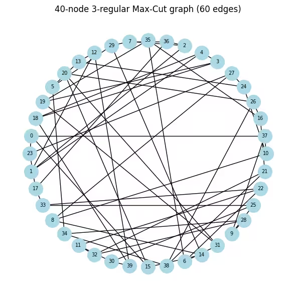
N_LARGE = 40
G_large = nx.random_regular_graph(d=3, n=N_LARGE, seed=0)
edges_large = list(G_large.edges())
print(f"Graph: {N_LARGE} nodes, {len(edges_large)} edges (3-regular)")

# Visualize the graph so it is clear what problem we are solving before any
# quantum work. Nodes in a circular layout; each edge contributes +1 to the
# cut value when its endpoints land in different partitions.
pos_large = nx.circular_layout(G_large)
fig, ax = plt.subplots(figsize=(6, 6))
nx.draw(
    G_large,
    pos_large,
    with_labels=True,
    node_color="lightblue",
    node_size=400,
    font_size=7,
    ax=ax,
)
ax.set_title(f"40-node 3-regular Max-Cut graph ({len(edges_large)} edges)")
plt.tight_layout()
plt.show()

# Same Maxcut → OptimizationProblem → QUBO → Ising pipeline as the small example,
# applied to the 40-node graph.
prob_large = Maxcut(G_large).to_optimization_problem()
converter_large = OptimizationProblemToQubo()
qubo_large = converter_large.convert(prob_large)
cost_op_large, offset_large = to_ising(qubo_large)
n_qubits_large = cost_op_large.num_qubits
print(
    f"Cost operator: {n_qubits_large} qubits, {len(cost_op_large)} Pauli terms"
)

# ── Step 1b: QP relaxation (multi-start L-BFGS-B) ─────────────────────────
# Same multi-start approach as the small example. At 40 qubits the relaxed
# landscape has many more local minima, so 200 random starts are essential
# to find a low-energy warm-start point.
Q_large = qubo_large.objective.quadratic.to_array(symmetric=True)
mu_large = qubo_large.objective.linear.to_array()

def qp_obj_large(x):
    return x @ Q_large @ x + mu_large @ x + qubo_large.objective.constant

bounds_large = [(0.0, 1.0)] * n_qubits_large
rng_qp = np.random.default_rng(42)
best_val_large, c_star_large = np.inf, None

for _ in range(200):
    x0 = rng_qp.uniform(0.0, 1.0, n_qubits_large)
    res = minimize(qp_obj_large, x0, method="L-BFGS-B", bounds=bounds_large)
    if res.fun < best_val_large:
        best_val_large, c_star_large = res.fun, res.x

# Regularize and convert to rotation angles (same formula as small example)
epsilon_large = 0.25
c_clipped_large = np.clip(c_star_large, epsilon_large, 1 - epsilon_large)
thetas_large = 2 * np.arcsin(np.sqrt(c_clipped_large))
print(
    f"c* range: [{c_star_large.min():.3f}, {c_star_large.max():.3f}]  "
    f"theta range: [{thetas_large.min():.3f}, {thetas_large.max():.3f}] rad"
)

# Plot the distribution of c* values to see how much structure the relaxation
# extracted. Values near 0/1 mean confident assignments; values near 0.5 mean
# the classical solver was uncertain and quantum exploration is most needed there.
fig, ax = plt.subplots(figsize=(6, 3))
ax.hist(c_star_large, bins=20, color="steelblue", edgecolor="white")
ax.axvline(0.5, color="k", linestyle="--", label="Uniform prior (std QAOA)")
ax.set_xlabel(r"$c^*_i$")
ax.set_ylabel("Count")
ax.set_title(r"Distribution of warm-start values $c^*_i$ (40-node graph)")
ax.legend()
plt.tight_layout()
plt.show()

# ── Step 1c: Build WS-QAOA circuit ─────────────────────────────────────────
# Reuse build_ws_qaoa from the small-scale section unchanged; the helper
# scales automatically with n_qubits and the cost operator size.
p_large = 1
ws_qc_large, ws_gammas_large, ws_betas_large = build_ws_qaoa(
    cost_op_large, p_large, n_qubits_large, thetas_large
)
ws_qc_large.measure_all()

# ── Step 2: Transpile to hardware-native gates ──────────────────────────
# generate_preset_pass_manager compiles the abstract circuit to th
# gate set of the backend and inserts SWAP gates wherever the cost Hamiltonian
# couples qubits that are not directly connected on the processor.
pm = generate_preset_pass_manager(optimization_level=3, backend=backend)
ws_isa_large = pm.run(ws_qc_large)

ecr_count = ws_isa_large.count_ops().get("ecr", 0)
print(
    f"\nTranspiled circuit: 2Q depth={ws_isa_large.depth(lambda x: x.operation.num_qubits == 2)}"
)
ws_isa_large.draw("mpl", fold=-1)

Graph: 40 nodes, 60 edges (3-regular)

Cost operator: 40 qubits, 60 Pauli terms
c* range: [0.000, 1.000]  theta range: [1.047, 2.094] rad

Transpiled circuit: 2Q depth=86

# ── Classical baseline via simulated annealing ────────────────────
# Run SA before any hardware calls to get a strong classical reference cut
# value. SA is fast (seconds), needs no solver license, and reliably finds
# near-optimal solutions on 40-node graphs. We use sa_cut as the denominator
# for the approximation ratio instead of the looser QP upper bound.
#
# At each step we flip a random node and accept the move if it improves the
# cut, or with probability exp(delta/T) otherwise. Temperature T decays
# geometrically, allowing uphill moves early on to escape local minima.
def simulated_annealing_maxcut(
    G, seed=0, T0=2.0, T_min=1e-4, alpha=0.995, n_steps=100_000
):
    rng_sa = np.random.default_rng(seed)
    n = G.number_of_nodes()
    x = rng_sa.integers(0, 2, n)
    best_x = x.copy()
    best_cut = sum(1 for u, v in G.edges() if x[u] != x[v])
    T = T0
    for _ in range(n_steps):
        i = rng_sa.integers(0, n)
        delta = sum((-1 if x[i] != x[nb] else 1) for nb in G.neighbors(i))
        if delta > 0 or rng_sa.random() < np.exp(delta / T):
            x[i] ^= 1
            cut = sum(1 for u, v in G.edges() if x[u] != x[v])
            if cut > best_cut:
                best_cut, best_x = cut, x.copy()
        T = max(T * alpha, T_min)
    return best_x, best_cut

sa_solution, sa_cut = simulated_annealing_maxcut(G_large)
print(f"Simulated annealing cut value: {sa_cut}  (classical reference)")

# ── Step 3: Execution on hardware ───────────────────────────
# A Session reserves the backend so the COBYLA iterations and final sampling
# run back-to-back without re-queuing between jobs — important when the
# optimizer submits many short jobs sequentially. All jobs are tagged with
# "TUT_WSQAOA" for traceability in the IBM Quantum dashboard.
#
# EstimatorV2 with resilience_level=1 enables twirled readout error extinction
# (TREX), which corrects systematic measurement bit-flip errors without extra
# circuit overhead. 4096 shots per call balances estimation noise vs. job time.
estimator_options = EstimatorOptions()
estimator_options.resilience_level = 1
estimator_options.default_shots = 4096
estimator_options.environment.job_tags = ["TUT_WSQAOA"]

# Align the cost observable with the physical qubit layout chosen by the transpiler
cost_op_isa = cost_op_large.apply_layout(ws_isa_large.layout)
ws_param_order_isa = list(ws_isa_large.parameters)

ws_history_hw = []

with Session(backend=backend) as session:
    estimator_hw = Estimator(mode=session, options=estimator_options)

    def hw_cost_fn(params):
        bound = ws_isa_large.assign_parameters(
            dict(zip(ws_param_order_isa, params))
        )
        energy = (
            estimator_hw.run([(bound, cost_op_isa)]).result()[0].data.evs.real
        )
        ws_history_hw.append(float(energy))
        print(
            f"  iter {len(ws_history_hw):>3d}  <H_C> = {energy:.4f}", end="\r"
        )
        return float(energy)

    # Warm-start initialization: gamma=0 means the cost unitary is the identity on
    # the first call, so COBYLA immediately evaluates the warm-start state itself —
    # a much better starting signal than a random point.
    ws_params0_hw = np.concatenate(
        [np.zeros(p_large), np.full(p_large, np.pi / 4)]
    )

    ws_result_hw = minimize(
        hw_cost_fn,
        ws_params0_hw,
        method="COBYLA",
        options={"maxiter": 150, "rhobeg": 0.3},
    )
    print(
        f"\nOptimization complete: energy={ws_result_hw.fun:.4f}, "
        f"iterations={len(ws_history_hw)}"
    )

    # ── Step 3b: Sample the optimized circuit ──────────────────────────────────
    # Use 8192 shots for the final sample to get a reliable mode estimate.
    sampler_hw = Sampler(
        mode=session,
        options={"environment": {"job_tags": ["TUT_WSQAOA"]}},
    )
    ws_bound_hw = ws_isa_large.assign_parameters(
        dict(zip(ws_param_order_isa, ws_result_hw.x))
    )
    counts_hw = (
        sampler_hw.run([ws_bound_hw], shots=8192)
        .result()[0]
        .data.meas.get_counts()
    )

best_bs_hw = max(counts_hw, key=counts_hw.get)
best_count = counts_hw[best_bs_hw]
total_shots = sum(counts_hw.values())

# Decode: Qiskit returns bitstrings with qubit 0 at the rightmost position,
# so reversing the string maps character index i to variable x_i.
cut_val_hw, s0_hw, s1_hw = evaluate_cut(best_bs_hw[::-1], G_large)

# Compare against simulated annealing.
# A ratio >= 1.0 means WS-QAOA matched or beat the classical SA solution.
# A ratio close to 1.0 (e.g. > 0.95) shows the quantum result is competitive.
approx_ratio_hw = cut_val_hw / sa_cut
print(
    f"Most-probable bitstring frequency: {best_count}/{total_shots} "
    f"({100*best_count/total_shots:.1f}%)"
)
print(
    f"WS-QAOA cut: {cut_val_hw}  |  SA cut: {sa_cut}  "
    f"|  Approximation ratio vs SA: {approx_ratio_hw:.4f}"
)

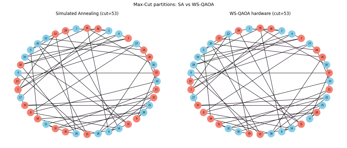
# Visualize both solutions side-by-side on the graph.
# Blue = partition S, orange = partition S-bar.
# Edges crossing between colors are the ones counted in the cut.
fig, axes = plt.subplots(1, 2, figsize=(14, 6))
for ax, assignment, cut, title in [
    (
        axes[0],
        list(sa_solution),
        sa_cut,
        f"Simulated Annealing (cut={sa_cut})",
    ),
    (
        axes[1],
        [int(b) for b in best_bs_hw[::-1]],
        cut_val_hw,
        f"WS-QAOA hardware (cut={cut_val_hw})",
    ),
]:
    colors = [
        "skyblue" if assignment[i] == 0 else "salmon" for i in G_large.nodes()
    ]
    nx.draw(
        G_large,
        pos_large,
        with_labels=True,
        node_color=colors,
        node_size=400,
        font_size=7,
        ax=ax,
    )
    ax.set_title(title)
plt.suptitle("Max-Cut partitions: SA vs WS-QAOA", fontsize=13)
plt.tight_layout()
plt.show()

# ── Step 4: Convergence plot and summary ──────────────────────────────────
# On real hardware the trace will be noisy (shot noise + gate errors), but the
# overall downward trend confirms that COBYLA is making progress despite noise.
fig, ax = plt.subplots(figsize=(7, 4))
ax.plot(ws_history_hw, color="tab:orange", label="WS-QAOA (hardware)")
ax.axhline(
    ws_result_hw.fun,
    color="tab:orange",
    linestyle=":",
    label=f"Final energy ({ws_result_hw.fun:.3f})",
)
ax.set_xlabel("Optimizer call")
ax.set_ylabel(r"$\langle H_C \rangle$")
ax.set_title(f"WS-QAOA convergence on {backend.name} (40 qubits, p=1)")
ax.legend()
plt.tight_layout()
plt.show()

print("\n=== Large Scale Summary ===")
print(f"{'Metric':<38} {'Value':>10}")
print("-" * 50)
print(f"{'Nodes / Edges':<38} {N_LARGE:>5} / {len(edges_large):<4}")
print(f"{'QAOA layers (p)':<38} {p_large:>10}")
print(f"{'Transpiled ECR gate count':<38} {ecr_count:>10}")
print(f"{'Transpiled circuit depth':<38} {ws_isa_large.depth():>10}")
print(f"{'Optimizer iterations':<38} {len(ws_history_hw):>10}")
print(f"{'WS-QAOA energy (hardware)':<38} {ws_result_hw.fun:>10.4f}")
print(f"{'Cut value':<38} {cut_val_hw:>10}")
print(f"{'Simulated annealing cut value':<38} {sa_cut:>10}")
print(f"{'Approximation ratio (vs SA)':<38} {approx_ratio_hw:>10.4f}")

Simulated annealing cut value: 53  (classical reference)
  iter  31  <H_C> = -12.4094
Optimization complete: energy=-13.0256, iterations=31
Most-probable bitstring frequency: 4/8192 (0.0%)
WS-QAOA cut: 53  |  SA cut: 53  |  Approximation ratio vs SA: 1.0000

=== Large Scale Summary ===
Metric                                      Value
--------------------------------------------------
Nodes / Edges                             40 / 60  
QAOA layers (p)                                 1
Transpiled ECR gate count                       0
Transpiled circuit depth                      276
Optimizer iterations                           31
WS-QAOA energy (hardware)                -13.0256
Cut value                                      53
Simulated annealing cut value                  53
Approximation ratio (vs SA)                1.0000

Próximos passos

Recommendations

Se você achou este trabalho interessante, talvez tenha interesse no seguinte material:

• Camadas QAOA mais altas: Aumente p para ver como ambos os algoritmos melhoram com mais camadas de circuito, e se a vantagem do WS-QAOA em profundidade baixa persiste.
• Qiskit addon optimization mapper: Explore a documentação e experimente modelar diferentes problemas combinatórios, ou usar diferentes solucionadores para a relaxação contínua.

Referências

[1] D. J. Egger, J. Mareček, and S. Woerner, "Warm-starting quantum optimization," Quantum, vol. 5, p. 479, 2021. arXiv:2009.10095

[2] E. Farhi, J. Goldstone, and S. Gutmann, "A quantum approximate optimization algorithm," arXiv:1411.4028, 2014.