Codificação de correlação de Pauli para reduzir requisitos de max-cut

Estimativa de uso: 35 minutos em um processador Eagle r3 (NOTA: Esta é apenas uma estimativa. Seu tempo de execução pode variar.)

Resultados de aprendizagem

Após concluir este tutorial, os usuários devem esperar os seguintes resultados:

• Compreender os princípios teóricos por trás da Codificação de Correlação de Pauli (PCE), incluindo como strings de Pauli de múltiplos corpos permitem a compressão polinomial de problemas de otimização clássicos.
• Implementar a PCE na prática para codificar e resolver tarefas de otimização em larga escala em hardware quântico de curto prazo.

Pré-requisitos

Recomendamos familiaridade com os seguintes tópicos antes de iniciar este tutorial:

• Algoritmos quânticos variacionais
• QAOA e max-cut

Contexto

Este tutorial apresenta a Codificação de Correlação de Pauli (PCE) [1], uma abordagem projetada para codificar problemas de otimização em qubits com maior eficiência para computação quântica. A PCE mapeia variáveis clássicas em problemas de otimização para correlações de matriz de Pauli de múltiplos corpos, resultando em uma compressão polinomial dos requisitos de espaço do problema. Ao empregar PCE, o número de qubits necessários para codificação é reduzido, tornando-a particularmente vantajosa para dispositivos quânticos de curto prazo com recursos limitados de qubits. Além disso, é demonstrado analiticamente que a PCE inerentemente mitiga platôs áridos, oferecendo resiliência super-polinomial contra este fenômeno. Este recurso integrado permite desempenho sem precedentes em solucionadores de otimização quântica.

Visão geral

A abordagem PCE consiste em três etapas principais, conforme ilustrado na Figura 1 de [1] a seguir:

1. Codificar o problema de otimização em um espaço de correlação de Pauli.
2. Resolver o problema usando um solucionador de otimização quântico-clássico.
3. Decodificar a solução de volta para o espaço de otimização original. A abordagem PCE é adaptável a qualquer solucionador de otimização quântica capaz de processar matrizes de correlação de Pauli. 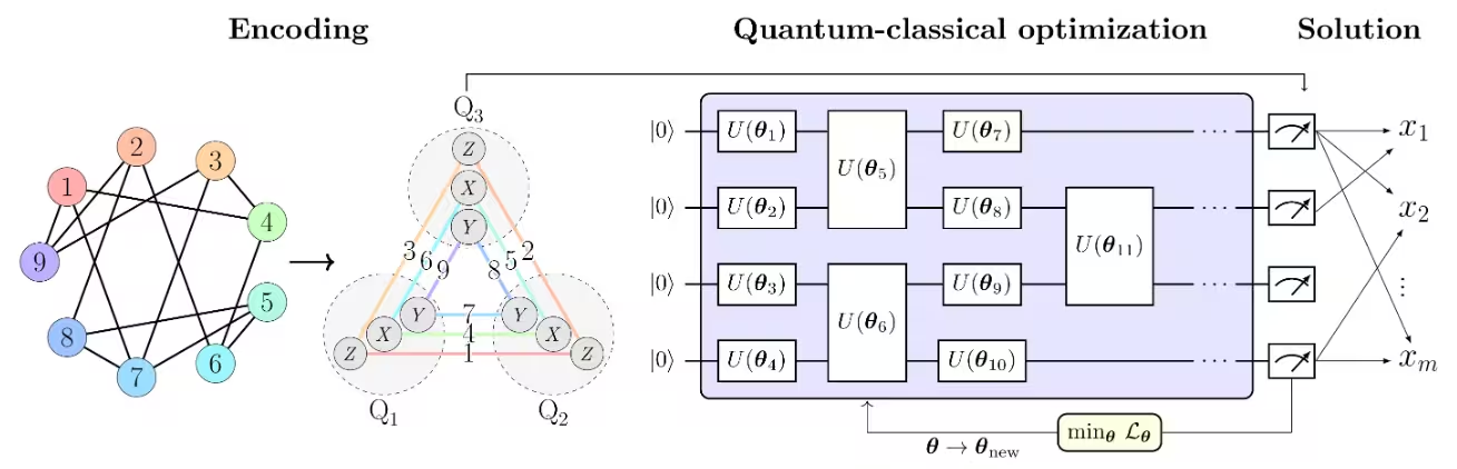Na Figura 1 de [1], o problema de max-cut é usado como exemplo para ilustrar a abordagem PCE. O problema de max-cut com $m=9$ nós é codificado em um espaço de correlação de Pauli, representando o problema de otimização como uma matriz de correlação — especificamente, correlações de matriz de Pauli de dois corpos através de $n=3$ qubits $(Q_1, Q_2, Q_3)$. As cores dos nós indicam a string de Pauli usada para cada nó codificado. Por exemplo, o nó 1, que corresponde à variável binária $x_1$, é codificado pelo valor esperado de $Z_1 \otimes Z_2 \otimes I_3$, enquanto $x_8$ é codificado por $I_1 \otimes Y_2 \otimes Y_3$. Isso corresponde a comprimir as $m$ variáveis do problema em $n = O(m^{1/2})$ qubits. De forma mais ampla, correlações de $k$ corpos permitem compressões polinomiais de ordem $k$, com $k>1$. O conjunto de Pauli escolhido compreende três subconjuntos de strings de Pauli mutuamente comutativas, permitindo que todas as $m$ correlações sejam estimadas experimentalmente com apenas três configurações de medição.

Uma função de perda $\mathcal{L}$ de valores esperados de Pauli que imita a função objetivo original do max-cut é construída. A função de perda é então otimizada usando um solucionador de otimização quântico-clássico, como o Variational Quantum Eigensolver (VQE).

Uma vez que a otimização está completa, a solução é decodificada de volta para o espaço de otimização original, produzindo a solução ótima do max-cut.

Requisitos

Antes de iniciar este tutorial, certifique-se de ter o seguinte instalado:

• Qiskit SDK v1.0 ou posterior, com suporte para visualização
• Qiskit Runtime v0.22 ou posterior (pip install qiskit-ibm-runtime)

Configuração

# Added by doQumentation — required packages for this notebook
!pip install -q networkx numpy qiskit qiskit-aer qiskit-ibm-runtime rustworkx scipy

from itertools import combinations

import numpy as np
import rustworkx as rx
import networkx as nx

from scipy.optimize import minimize, OptimizeResult

from qiskit.circuit.library import efficient_su2
from qiskit.transpiler.preset_passmanagers import generate_preset_pass_manager
from qiskit.quantum_info import SparsePauliOp
from qiskit_ibm_runtime import EstimatorV2 as Estimator
from qiskit_ibm_runtime import QiskitRuntimeService
from qiskit_ibm_runtime import Session
from rustworkx.visualization import mpl_draw
from qiskit_aer import AerSimulator

def calc_cut_size(graph, partition0, partition1):
    """Calculate the cut size of the given partitions of the graph."""

    cut_size = 0
    for edge0, edge1 in graph.edge_list():
        if edge0 in partition0 and edge1 in partition1:
            cut_size += 1
        elif edge0 in partition1 and edge1 in partition0:
            cut_size += 1
    return cut_size

Exemplo com simulador em pequena escala

service = QiskitRuntimeService()
real_backend = service.least_busy(
    operational=True, simulator=False, min_num_qubits=156
)
backend = AerSimulator.from_backend(real_backend)
print(f"We are using the {backend.name}")

We are using the aer_simulator_from(ibm_pittsburgh)

Passo 1: Mapear entradas clássicas para um problema quântico

O problema de max-cut

O problema de max-cut é um problema de otimização combinatória que é definido em um grafo $G = (V, E)$, onde $V$ é o conjunto de vértices e $E$ é o conjunto de arestas. O objetivo é particionar os vértices em dois conjuntos, $S$ e $V \setminus S$, de modo que o número de arestas entre os dois conjuntos seja maximizado. Para a descrição detalhada do problema de max-cut, consulte o tutorial Algoritmo de otimização aproximada quântica. O problema de max-cut também é usado como exemplo no tutorial Técnicas avançadas para QAOA. Nesses tutoriais, o algoritmo QAOA é usado para resolver o problema de max-cut.

Grafo -> Hamiltoniano

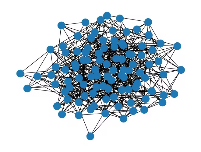
Vamos primeiro considerar um grafo aleatório com 100 nós.

num_nodes = 100  # Number of nodes in graph
seed = 42
graph = rx.undirected_gnp_random_graph(num_nodes, 0.1, seed=seed)
mpl_draw(graph)

nx_graph = nx.Graph()
nx_graph.add_nodes_from(range(num_nodes))

for edge in graph.edge_list():
    nx_graph.add_edge(edge[0], edge[1])

curr_cut_size, partition = nx.approximation.one_exchange(nx_graph, seed=1)
print(f"Initial cut size: {curr_cut_size}")

Initial cut size: 345

Codificamos o grafo com 100 nós em correlações de matriz de Pauli de dois corpos através de nove qubits (veja a explicação abaixo). O grafo é representado como uma matriz de correlação, onde cada nó é codificado por uma string de Pauli. O sinal do valor esperado da string de Pauli indica a partição do nó. Por exemplo, o nó 0 é codificado por uma string de Pauli, $\prod_0 = I_{8} \otimes ... I_2 \otimes X_1 \otimes X_0$. O sinal do valor esperado desta string de Pauli indica a partição do nó 0. Definimos uma codificação de correlação de Pauli (PCE) relativa a $\prod$ como

$x_i \coloneqq \textit{sgn}(\langle\prod_i \rangle),$

onde $x_i$ é a partição do nó $i$ e $\langle \prod_i \rangle \coloneqq \langle \psi |\prod_i| \psi \rangle$ é o valor esperado da string de Pauli codificando o nó $i$ sobre um estado quântico $|\psi \rangle$. Agora, vamos codificar o grafo em um Hamiltoniano usando PCE. Dividimos os nós em três conjuntos: $S_1$, $S_2$ e $S_3$. Então, codificamos os nós em cada conjunto usando as strings de Pauli com $X$, $Y$ e $Z$, respectivamente. Precisamos extrair uma relação entre o número de nós e qubits necessários para codificar todos os nós. Usando todas as permutações possíveis para a codificação, obtemos:

$$m=3\binom{n}{k}.$$

Neste exemplo consideramos $k=2$, portanto,

$$m = \frac{3}{2} n(n-1).$$

Portanto, o número de qubits $n$ necessários para expressar um certo número de nós $m$ é:

$$n = \left\lceil \frac{1 + \sqrt{1 + \tfrac{8}{3}m}}{2} \right\rceil.$$

Observe que o símbolo $\lceil \cdot \rceil$ representa a função teto, que arredonda qualquer número real para cima até o próximo inteiro. Isso garante que o número de qubits seja um inteiro.

num_qubits = int(np.ceil((1 + np.sqrt(1 + (8 / 3) * num_nodes)) / 2))

list_size = num_nodes // 3
node_x = [i for i in range(list_size)]
node_y = [i for i in range(list_size, 2 * list_size)]
node_z = [i for i in range(2 * list_size, num_nodes)]

print(f"Number of qubits: {num_qubits}")
print("List 1:", node_x)
print("List 2:", node_y)
print("List 3:", node_z)

Number of qubits: 9
List 1: [0, 1, 2, 3, 4, 5, 6, 7, 8, 9, 10, 11, 12, 13, 14, 15, 16, 17, 18, 19, 20, 21, 22, 23, 24, 25, 26, 27, 28, 29, 30, 31, 32]
List 2: [33, 34, 35, 36, 37, 38, 39, 40, 41, 42, 43, 44, 45, 46, 47, 48, 49, 50, 51, 52, 53, 54, 55, 56, 57, 58, 59, 60, 61, 62, 63, 64, 65]
List 3: [66, 67, 68, 69, 70, 71, 72, 73, 74, 75, 76, 77, 78, 79, 80, 81, 82, 83, 84, 85, 86, 87, 88, 89, 90, 91, 92, 93, 94, 95, 96, 97, 98, 99]

def build_pauli_correlation_encoding(pauli, node_list, n, k=2):
    pauli_correlation_encoding = []
    for idx, c in enumerate(combinations(range(n), k)):
        if idx >= len(node_list):
            break
        paulis = ["I"] * n
        paulis[c[0]], paulis[c[1]] = pauli, pauli
        pauli_correlation_encoding.append(("".join(paulis)[::-1], 1))

    hamiltonian = []
    for pauli, weight in pauli_correlation_encoding:
        hamiltonian.append(SparsePauliOp.from_list([(pauli, weight)]))

    return hamiltonian

pauli_correlation_encoding_x = build_pauli_correlation_encoding(
    "X", node_x, num_qubits
)
pauli_correlation_encoding_y = build_pauli_correlation_encoding(
    "Y", node_y, num_qubits
)
pauli_correlation_encoding_z = build_pauli_correlation_encoding(
    "Z", node_z, num_qubits
)

Passo 2: Otimizar o problema para execução em hardware quântico

Circuito quântico

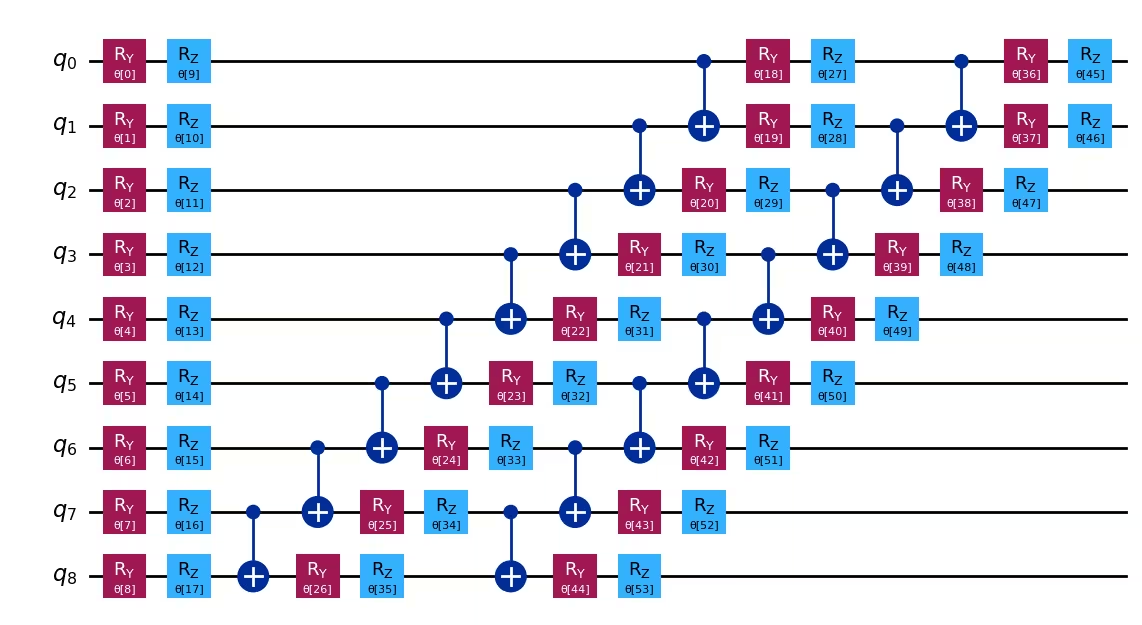
Aqui, o estado $|\psi \rangle$ é parametrizado com $\mathbf{\theta}$, e otimizamos esses parâmetros $\mathbf{\theta}$ usando uma abordagem variacional. Este tutorial emprega o ansatz efficient_su2 para nosso algoritmo variacional devido às suas capacidades expressivas e facilidade de implementação. Também usamos a função de perda relaxada, que será introduzida mais adiante neste tutorial. Como resultado, podemos abordar problemas de larga escala com menos qubits e profundidades de circuito mais rasas.

# Build the quantum circuit
qc = efficient_su2(num_qubits, su2_gates=["ry", "rz"], reps=2)
qc.draw("mpl")

# Optimize the circuit

pm = generate_preset_pass_manager(optimization_level=3, backend=backend)
qc = pm.run(qc)

Função de perda

Para a função de perda $\mathcal{L}$, usamos uma relaxação da função objetivo do max-cut conforme descrito em [1], que é definida como $\mathcal{V}(\mathbf{x}) \coloneqq \sum_{(i, j) \in E} W_{i, j}(1-x_i x_j)$. Aqui, $W_{i, j}$ denota o peso da aresta $(i, j)$, e $x_i$ representa a partição do nó $i$. A função de perda $\mathcal{L}$ é dada por:

$\mathcal{L}\coloneqq \sum_{(i, j) \in E} W_{i, j} \text{tanh} (\alpha \langle\prod_i \rangle) \text{tanh} (\alpha \langle\prod_j \rangle) + \mathcal{L}^{(\text{reg})},$

onde a função objetivo do max-cut é substituída pelas tangentes hiperbólicas suaves dos valores esperados das strings de Pauli codificando os nós. O termo de regularização $\mathcal{L}^{(\text{reg})}$ e o fator de reescala $\alpha$, proporcional ao número de qubits, são introduzidos para melhorar o desempenho do solucionador.

O termo de regularização é definido como:

$\mathcal{L}^{(\text{reg})}$ é definido como $\mathcal{L}^{(\text{reg})} \coloneqq \beta \nu \lbrack \frac{1}{m} \sum_{i \in V} \text{tanh} (\alpha \langle\prod_i \rangle)^2 \rbrack ^2$

onde $\beta=1/2$, $\nu = |E|/2 + (m -1) /4$, $|E|$ é o número de arestas, e $m$ é o número de nós no grafo.

def loss_func_estimator(x, ansatz, hamiltonian, estimator, graph):
    """
    Calculates the specified loss function for the given ansatz, Hamiltonian,
    and graph.

    The expectation values of each Pauli string in the Hamiltonian are first
    obtained by running the ansatz on the quantum backend. These
    expectation values are then passed through the nonlinear function
    tanh(alpha * prod_i). The loss function is
    subsequently computed from these transformed values.
    """
    job = estimator.run(
        [
            (ansatz, hamiltonian[0], x),
            (ansatz, hamiltonian[1], x),
            (ansatz, hamiltonian[2], x),
        ]
    )
    result = job.result()

    # calculate the loss function
    node_exp_map = {}
    idx = 0
    for r in result:
        for ev in r.data.evs:
            node_exp_map[idx] = ev
            idx += 1

    loss = 0
    alpha = num_qubits
    for edge0, edge1 in graph.edge_list():
        loss += np.tanh(alpha * node_exp_map[edge0]) * np.tanh(
            alpha * node_exp_map[edge1]
        )

    regulation_term = 0
    for i in range(len(graph.nodes())):
        regulation_term += np.tanh(alpha * node_exp_map[i]) ** 2
    regulation_term = regulation_term / len(graph.nodes())
    regulation_term = regulation_term**2
    beta = 1 / 2
    v = len(graph.edges()) / 2 + (len(graph.nodes()) - 1) / 4
    regulation_term = beta * v * regulation_term

    loss = loss + regulation_term

    global experiment_result
    print(f"Iter {len(experiment_result)}: {loss}")
    experiment_result.append({"loss": loss, "exp_map": node_exp_map})
    return loss

Passo 3: Executar usando primitivas Qiskit

Neste tutorial, definimos max_iter=50 no loop de otimização para fins de demonstração. Se aumentarmos o número de iterações, podemos esperar melhores resultados.

pce = []
pce.append(
    [op.apply_layout(qc.layout) for op in pauli_correlation_encoding_x]
)
pce.append(
    [op.apply_layout(qc.layout) for op in pauli_correlation_encoding_y]
)
pce.append(
    [op.apply_layout(qc.layout) for op in pauli_correlation_encoding_z]
)

max_iter = 50
counter = {"i": 0}
last_x = {"value": None}
last_fun = {"value": None}

with Session(backend=backend) as session:
    estimator = Estimator(mode=session)

    experiment_result = []

    def loss_func(x):
        last_x["value"] = x.copy()
        if counter["i"] + 1 > max_iter:
            return last_fun["value"]
        counter["i"] += 1
        val = loss_func_estimator(
            x, qc, [pce[0], pce[1], pce[2]], estimator, graph
        )
        last_fun["value"] = val
        return val

    np.random.seed(seed)
    initial_params = np.random.rand(qc.num_parameters)

    result = minimize(
        loss_func, initial_params, method="COBYLA", options={"rhobeg": 1.0}
    )

    if counter["i"] >= max_iter:
        result = OptimizeResult(
            message=f"Return from COBYLA because the objective function "
            f"has been evaluated {max_iter} times.",
            success=False,
            status=3,
            fun=last_fun["value"],
            x=last_x["value"],
            nfev=counter["i"],
        )

print(result)

Iter 0: 159.88755362682548
Iter 1: 113.46202580636677
Iter 2: 56.76494226400048
Iter 3: 32.63357946896002
Iter 4: 21.517837239610117
Iter 5: 30.96034960483569
Iter 6: 20.780475923938027
Iter 7: 24.54251816279811
Iter 8: 27.834486461763042
Iter 9: 16.705460776812693
Iter 10: 18.020587887236864
Iter 11: 12.252379762741352
Iter 12: 5.253885750886939
Iter 13: 6.985984759592262
Iter 14: 6.908717244584757
Iter 15: 12.915466016863858
Iter 16: 4.105776920457279
Iter 17: 11.707504530740305
Iter 18: 7.154360511076546
Iter 19: 10.3890865704735
Iter 20: 10.376147647857252
Iter 21: 2.533430195296697
Iter 22: 3.8612421907795462
Iter 23: 6.103735057461906
Iter 24: -1.1190368234312347
Iter 25: 6.125915279494738
Iter 26: 11.086280445482455
Iter 27: 10.102569882302827
Iter 28: -0.02664415648133822
Iter 29: 7.621887727398785
Iter 30: 5.967346615554497
Iter 31: 3.85345716014828
Iter 32: 4.5494846149011
Iter 33: 10.006668112637232
Iter 34: -3.1927138938527877
Iter 35: 2.8829882366285116
Iter 36: 3.3130087521654144
Iter 37: -4.907566569808272
Iter 38: -4.980134722109894
Iter 39: -2.990457463896541
Iter 40: -5.938401817344579
Iter 41: -2.1807712386469724
Iter 42: -1.0945774380342126
Iter 43: -4.7548102593556685
Iter 44: -3.8762362299208144
Iter 45: -4.9348321021624
Iter 46: -6.487722842864011
Iter 47: 0.7064210113389331
Iter 48: -2.3428323031772216
Iter 49: -2.626032270380895
 message: Return from COBYLA because the objective function has been evaluated 50 times.
 success: False
  status: 3
     fun: -2.626032270380895
       x: [ 1.375e+00  1.951e+00 ...  9.395e-01  8.948e-01]
    nfev: 50

Passo 4: Pós-processar e retornar resultado no formato clássico desejado

As partições dos nós são determinadas avaliando o sinal dos valores esperados das strings de Pauli que codificam os nós.

# Calculate the partitions based on the final expectation values
# If the expectation value is positive, the node belongs to partition 0 (par0)
# Otherwise, the node belongs to partition 1 (par1)
def get_partitions(experiment_result):
    par0, par1 = set(), set()
    best_index = min(
        range(len(experiment_result)),
        key=lambda i: experiment_result[i]["loss"],
    )
    for i in experiment_result[best_index]["exp_map"]:
        if experiment_result[best_index]["exp_map"][i] >= 0:
            par0.add(i)
        else:
            par1.add(i)
    return par0, par1, best_index

par0, par1, best_index = get_partitions(experiment_result)
print(par0, par1)

{0, 2, 3, 8, 9, 11, 12, 13, 17, 18, 20, 22, 23, 24, 25, 26, 27, 30, 35, 37, 38, 40, 43, 46, 48, 49, 50, 51, 53, 57, 61, 62, 63, 66, 67, 68, 70, 71, 74, 77, 81, 82, 83, 84, 87, 88, 94, 96, 99} {1, 4, 5, 6, 7, 10, 14, 15, 16, 19, 21, 28, 29, 31, 32, 33, 34, 36, 39, 41, 42, 44, 45, 47, 52, 54, 55, 56, 58, 59, 60, 64, 65, 69, 72, 73, 75, 76, 78, 79, 80, 85, 86, 89, 90, 91, 92, 93, 95, 97, 98}

Podemos calcular o tamanho do corte do problema de max-cut usando as partições dos nós.

cut_size = calc_cut_size(graph, par0, par1)
print(f"Cut size: {cut_size}")

Cut size: 268

Uma vez que o treinamento está completo, realizamos uma rodada de busca de troca de bit único para melhorar a solução como uma etapa de pós-processamento clássico. Neste processo, trocamos as partições de dois nós e avaliamos o tamanho do corte. Se o tamanho do corte for melhorado, mantemos a troca. Repetimos este processo para todos os pares possíveis de nós conectados por uma aresta.

cur_bits = []

for i in experiment_result[best_index]["exp_map"]:
    if experiment_result[best_index]["exp_map"][i] >= 0:
        cur_bits.append(1)
    else:
        cur_bits.append(0)
print(cur_bits)

[1, 0, 1, 1, 0, 0, 0, 0, 1, 1, 0, 1, 1, 1, 0, 0, 0, 1, 1, 0, 1, 0, 1, 1, 1, 1, 1, 1, 0, 0, 1, 0, 0, 0, 0, 1, 0, 1, 1, 0, 1, 0, 0, 1, 0, 0, 1, 0, 1, 1, 1, 1, 0, 1, 0, 0, 0, 1, 0, 0, 0, 1, 1, 1, 0, 0, 1, 1, 1, 0, 1, 1, 0, 0, 1, 0, 0, 1, 0, 0, 0, 1, 1, 1, 1, 0, 0, 1, 1, 0, 0, 0, 0, 0, 1, 0, 1, 0, 0, 1]

# Swap the partitions and calculate the cut size

def swap_partitions(graph, cur_bits):
    best_cut = 0
    best_bits = []
    for edge0, edge1 in graph.edge_list():
        swapped_bits = cur_bits.copy()
        swapped_bits[edge0], swapped_bits[edge1] = (
            swapped_bits[edge1],
            swapped_bits[edge0],
        )

        cur_partition = [set(), set()]
        for i, bit in enumerate(swapped_bits):
            if bit > 0:
                cur_partition[0].add(i)
            else:
                cur_partition[1].add(i)
        cut_size = calc_cut_size(graph, cur_partition[0], cur_partition[1])
        if best_cut < cut_size:
            best_cut = cut_size
            best_bits = swapped_bits
    return best_cut, best_bits

best_cut, best_bits = swap_partitions(graph, cur_bits)
print(best_cut, best_bits)

279 [1, 0, 1, 1, 0, 0, 0, 0, 1, 0, 0, 1, 1, 1, 0, 0, 0, 1, 1, 0, 1, 0, 1, 1, 1, 1, 1, 1, 0, 0, 1, 0, 0, 0, 0, 1, 0, 1, 1, 0, 1, 0, 0, 1, 0, 0, 1, 0, 1, 1, 1, 1, 1, 1, 0, 0, 0, 1, 0, 0, 0, 1, 1, 1, 0, 0, 1, 1, 1, 0, 1, 1, 0, 0, 1, 0, 0, 1, 0, 0, 0, 1, 1, 1, 1, 0, 0, 1, 1, 0, 0, 0, 0, 0, 1, 0, 1, 0, 0, 1]

Exemplo de hardware em larga escala

# -------------------------Step 1-------------------------

num_nodes = 1500  # Number of nodes in graph
graph = rx.undirected_gnp_random_graph(num_nodes, 0.1, seed=seed)
nx_graph = nx.Graph()
nx_graph.add_nodes_from(range(num_nodes))
for edge in graph.edge_list():
    nx_graph.add_edge(edge[0], edge[1])

num_qubits = int(np.ceil((1 + np.sqrt(1 + (8 / 3) * num_nodes)) / 2))

list_size = num_nodes // 3
node_x = [i for i in range(list_size)]
node_y = [i for i in range(list_size, 2 * list_size)]
node_z = [i for i in range(2 * list_size, num_nodes)]

pauli_correlation_encoding_x = build_pauli_correlation_encoding(
    "X", node_x, num_qubits
)
pauli_correlation_encoding_y = build_pauli_correlation_encoding(
    "Y", node_y, num_qubits
)
pauli_correlation_encoding_z = build_pauli_correlation_encoding(
    "Z", node_z, num_qubits
)
print(f"We are using {num_qubits} qubits")

# -------------------------Step 2-------------------------
backend = real_backend
print(f"We are using the {backend.name}")
qc = efficient_su2(num_qubits, ["ry", "rz"], reps=2)
pm = generate_preset_pass_manager(optimization_level=3, backend=backend)
qc = pm.run(qc)
# -------------------------Step 3-------------------------
pce = []
pce.append(
    [op.apply_layout(qc.layout) for op in pauli_correlation_encoding_x]
)
pce.append(
    [op.apply_layout(qc.layout) for op in pauli_correlation_encoding_y]
)
pce.append(
    [op.apply_layout(qc.layout) for op in pauli_correlation_encoding_z]
)

# Run the optimization using a session.
max_iter = 50
counter = {"i": 0}
with Session(backend=backend) as session:
    estimator = Estimator(mode=session)
    estimator.options.environment.job_tags = ["TUT_PCEFQ"]
    experiment_result = []

    def loss_func(x):
        last_x["value"] = x.copy()
        if counter["i"] + 1 > max_iter:
            return last_fun["value"]
        counter["i"] += 1
        val = loss_func_estimator(
            x, qc, [pce[0], pce[1], pce[2]], estimator, graph
        )
        last_fun["value"] = val
        return val

    np.random.seed(seed)
    initial_params = np.random.rand(qc.num_parameters)
    result = minimize(
        loss_func, initial_params, method="COBYLA", options={"rhobeg": 1.0}
    )
    if counter["i"] >= max_iter:
        result = OptimizeResult(
            message="Return from COBYLA because the objective function "
            "has been evaluated {max_iter} times.",
            success=False,
            status=3,
            fun=last_fun["value"],
            x=last_x["value"],
            nfev=counter["i"],
        )
print(result)

# -------------------------Step 4-------------------------

par0, par1, best_index = get_partitions(experiment_result)
cut_size = calc_cut_size(graph, par0, par1)
print(f"Cut size: {cut_size}")

best_bits = []
cur_bits = []
for i in experiment_result[best_index]["exp_map"]:
    if experiment_result[best_index]["exp_map"][i] >= 0:
        cur_bits.append(1)
    else:
        cur_bits.append(0)
best_cut, best_bits = swap_partitions(graph, cur_bits)
# Print final solution

print(
    f"The best max-cut value achieved for a graph with {num_nodes} nodes "
    f"on {num_qubits} qubits is {best_cut}"
)
print(f"and the specific partition we obtained is {best_bits}")

We are using 33 qubits
We are using the ibm_pittsburgh
Iter 0: 57399.57543902076
Iter 1: 56458.787143794
Iter 2: 40778.45608998947
Iter 3: 35571.58511146131
Iter 4: 33861.6835761173
Iter 5: 39697.22637736274
Iter 6: 34984.77893767163
Iter 7: 32051.882157096858
Iter 8: 26134.153216063707
Iter 9: 24914.322627065787
Iter 10: 24030.21227315425
Iter 11: 23047.463945514
Iter 12: 22629.42866110748
Iter 13: 17374.859132614685
Iter 14: 18020.11637762458
Iter 15: 17924.7066364044
Iter 16: 15825.1992250984
Iter 17: 16553.346711978447
Iter 18: 12393.565736512377
Iter 19: 11994.021456089155
Iter 20: 11199.994322735669
Iter 21: 9624.895532927634
Iter 22: 9073.811130188606
Iter 23: 9836.721241931278
Iter 24: 10555.925186133794
Iter 25: 9179.1179493286
Iter 26: 8495.394826965305
Iter 27: 8913.688189840399
Iter 28: 7830.448471810181
Iter 29: 7757.430542422075
Iter 30: 6796.187594518731
Iter 31: 7307.985913766867
Iter 32: 7340.225833330675
Iter 33: 7064.731899380469
Iter 34: 7632.270657372515
Iter 35: 7049.154710767935
Iter 36: 7486.118442084411
Iter 37: 6302.12602219333
Iter 38: 6244.934230209166
Iter 39: 7154.9748739261395
Iter 40: 6482.109600054041
Iter 41: 5718.475169152395
Iter 42: 5693.008457857462
Iter 43: 4869.782667921923
Iter 44: 4957.625304450959
Iter 45: 5582.240637063214
Iter 46: 4983.90082772116
Iter 47: 5416.268575648202
Iter 48: 4809.98398457807
Iter 49: 5092.527306646118
 message: Return from COBYLA because the objective function has been evaluated 50 times.
 success: False
  status: 3
     fun: 5092.527306646118
       x: [ 1.375e+00  1.951e+00 ...  7.259e-01  8.971e-01]
    nfev: 50
Cut size: 56152
The best max-cut value achieved for a graph with 1500 nodes on 33 qubits is 56219
and the specific partition we obtained is [1, 0, 0, 0, 1, 1, 0, 1, 1, 0, 0, 0, 0, 0, 1, 1, 0, 1, 0, 0, 1, 0, 0, 1, 1, 1, 0, 1, 1, 0, 1, 0, 1, 1, 0, 0, 0, 0, 0, 1, 0, 1, 0, 0, 1, 0, 0, 0, 1, 0, 1, 1, 1, 1, 0, 1, 0, 0, 1, 0, 0, 0, 0, 1, 1, 0, 0, 0, 0, 1, 1, 1, 1, 1, 0, 0, 0, 1, 0, 0, 1, 1, 0, 0, 1, 1, 1, 1, 1, 1, 0, 0, 0, 1, 0, 0, 0, 0, 1, 0, 1, 1, 1, 1, 1, 0, 1, 0, 0, 1, 0, 0, 0, 0, 0, 0, 1, 0, 0, 0, 1, 0, 1, 1, 1, 1, 0, 1, 1, 1, 1, 0, 0, 0, 1, 0, 0, 0, 1, 1, 0, 1, 1, 0, 1, 0, 0, 1, 1, 1, 1, 1, 1, 0, 1, 0, 1, 0, 0, 0, 0, 0, 0, 1, 0, 1, 0, 0, 1, 1, 1, 0, 1, 0, 1, 0, 0, 1, 1, 0, 1, 0, 1, 0, 0, 0, 1, 0, 1, 0, 1, 1, 1, 1, 1, 0, 1, 0, 1, 1, 1, 1, 1, 1, 0, 0, 0, 0, 0, 1, 0, 1, 0, 0, 1, 1, 0, 0, 1, 0, 1, 0, 1, 0, 0, 0, 0, 0, 1, 1, 0, 0, 0, 0, 0, 1, 1, 0, 0, 1, 1, 1, 1, 1, 1, 1, 0, 1, 1, 1, 1, 0, 1, 1, 0, 1, 0, 0, 1, 1, 1, 0, 1, 0, 1, 1, 1, 0, 1, 0, 0, 0, 1, 1, 1, 1, 1, 1, 0, 1, 0, 0, 0, 0, 1, 1, 1, 1, 1, 1, 1, 0, 0, 1, 1, 1, 1, 0, 1, 0, 0, 1, 1, 1, 0, 1, 0, 1, 1, 1, 1, 0, 1, 1, 0, 1, 0, 0, 0, 0, 0, 0, 0, 0, 0, 0, 1, 0, 0, 0, 0, 0, 0, 1, 1, 1, 0, 0, 1, 1, 1, 0, 1, 0, 1, 0, 1, 0, 1, 1, 1, 0, 0, 1, 1, 1, 0, 1, 0, 0, 0, 1, 1, 1, 0, 0, 0, 1, 0, 1, 0, 0, 0, 0, 1, 1, 0, 0, 1, 1, 1, 1, 0, 1, 0, 1, 0, 0, 1, 1, 0, 0, 1, 1, 0, 0, 0, 1, 1, 1, 0, 1, 1, 0, 0, 0, 1, 1, 1, 0, 0, 1, 1, 1, 1, 1, 0, 0, 1, 1, 0, 0, 0, 0, 0, 0, 1, 1, 1, 1, 1, 1, 1, 0, 0, 0, 1, 1, 0, 0, 0, 1, 0, 0, 1, 0, 0, 1, 0, 1, 1, 0, 0, 0, 0, 0, 0, 0, 1, 1, 1, 1, 1, 0, 0, 0, 1, 0, 0, 1, 1, 1, 1, 1, 1, 1, 1, 1, 1, 1, 0, 1, 0, 1, 1, 1, 1, 1, 0, 0, 0, 1, 1, 1, 0, 1, 1, 1, 1, 0, 0, 1, 0, 1, 0, 1, 1, 0, 0, 0, 1, 0, 1, 0, 1, 1, 1, 0, 1, 0, 1, 1, 0, 1, 1, 0, 1, 1, 1, 0, 0, 1, 1, 1, 0, 1, 0, 1, 0, 1, 0, 0, 0, 1, 1, 0, 1, 0, 0, 1, 0, 0, 1, 0, 0, 0, 0, 0, 1, 0, 0, 0, 0, 0, 1, 0, 0, 0, 0, 0, 0, 0, 0, 1, 0, 1, 0, 0, 1, 0, 1, 0, 0, 0, 0, 1, 0, 0, 0, 1, 1, 1, 1, 1, 0, 0, 1, 0, 1, 1, 1, 1, 0, 1, 1, 0, 1, 0, 0, 0, 0, 1, 0, 0, 1, 1, 0, 1, 0, 1, 0, 1, 0, 0, 1, 0, 0, 0, 1, 1, 1, 0, 0, 1, 0, 0, 1, 0, 1, 0, 1, 1, 1, 1, 0, 1, 1, 1, 0, 1, 1, 1, 1, 1, 1, 1, 1, 0, 1, 0, 1, 1, 1, 0, 0, 0, 1, 0, 0, 0, 0, 0, 1, 0, 0, 1, 0, 1, 1, 1, 0, 0, 0, 0, 0, 0, 1, 0, 1, 1, 0, 1, 1, 1, 1, 0, 0, 1, 1, 0, 1, 1, 1, 0, 1, 0, 1, 0, 1, 0, 0, 0, 0, 0, 0, 0, 0, 1, 0, 0, 1, 1, 1, 0, 1, 1, 0, 0, 0, 1, 0, 1, 0, 1, 1, 1, 0, 1, 1, 1, 0, 1, 1, 1, 1, 0, 0, 1, 1, 0, 1, 1, 1, 0, 0, 0, 0, 0, 0, 0, 1, 1, 1, 1, 1, 0, 1, 0, 1, 0, 1, 0, 0, 0, 1, 0, 1, 0, 1, 0, 1, 0, 1, 0, 1, 1, 1, 1, 1, 0, 0, 1, 0, 1, 0, 1, 0, 1, 1, 0, 1, 0, 1, 0, 0, 0, 1, 0, 0, 0, 1, 1, 1, 0, 1, 0, 0, 1, 0, 1, 0, 1, 0, 1, 0, 0, 1, 0, 1, 0, 0, 0, 1, 1, 1, 0, 1, 0, 0, 0, 0, 1, 0, 0, 0, 0, 1, 0, 0, 1, 1, 1, 0, 1, 1, 0, 1, 1, 1, 0, 0, 0, 0, 1, 0, 1, 0, 0, 0, 1, 0, 1, 0, 1, 0, 0, 1, 0, 1, 0, 1, 0, 1, 1, 0, 0, 1, 1, 0, 1, 1, 0, 0, 1, 0, 1, 1, 1, 0, 1, 1, 0, 1, 1, 1, 0, 1, 1, 0, 1, 0, 1, 0, 1, 1, 0, 1, 1, 0, 1, 1, 0, 0, 0, 1, 0, 1, 0, 0, 0, 0, 0, 1, 0, 0, 1, 1, 0, 1, 0, 1, 1, 0, 1, 1, 0, 1, 1, 1, 1, 0, 1, 0, 1, 1, 0, 0, 1, 0, 0, 1, 1, 0, 1, 1, 1, 0, 1, 1, 0, 1, 1, 1, 0, 1, 0, 0, 0, 1, 0, 0, 1, 1, 1, 0, 0, 1, 0, 1, 1, 1, 0, 1, 0, 1, 1, 1, 1, 1, 1, 0, 1, 0, 0, 0, 1, 0, 1, 0, 1, 1, 0, 0, 0, 1, 1, 0, 1, 1, 1, 1, 1, 1, 1, 1, 1, 1, 1, 1, 0, 1, 1, 1, 0, 0, 0, 0, 1, 0, 0, 0, 0, 1, 1, 1, 0, 0, 1, 0, 0, 0, 0, 0, 0, 0, 1, 0, 0, 0, 0, 0, 0, 0, 1, 1, 0, 0, 1, 0, 0, 1, 1, 0, 1, 0, 1, 0, 1, 0, 0, 1, 1, 0, 1, 1, 1, 0, 0, 1, 1, 1, 1, 1, 0, 0, 1, 0, 1, 1, 1, 1, 0, 1, 0, 1, 1, 0, 0, 1, 0, 1, 0, 0, 1, 0, 1, 1, 1, 1, 1, 1, 1, 0, 1, 0, 1, 1, 0, 0, 0, 0, 0, 1, 1, 0, 0, 1, 1, 1, 1, 1, 1, 1, 1, 1, 1, 0, 1, 1, 1, 1, 0, 1, 0, 0, 0, 1, 1, 1, 1, 0, 0, 0, 1, 1, 0, 0, 0, 0, 0, 1, 0, 0, 0, 1, 0, 0, 0, 1, 1, 1, 1, 0, 0, 0, 1, 1, 1, 1, 1, 1, 1, 1, 1, 1, 0, 1, 1, 1, 1, 1, 1, 1, 0, 0, 0, 0, 0, 1, 1, 0, 0, 0, 1, 1, 0, 0, 0, 0, 0, 1, 0, 0, 0, 0, 0, 0, 0, 0, 1, 0, 1, 0, 1, 1, 1, 0, 1, 0, 1, 1, 1, 1, 1, 0, 1, 1, 1, 1, 0, 1, 1, 1, 1, 1, 1, 0, 0, 1, 1, 0, 0, 1, 1, 1, 1, 1, 0, 1, 0, 1, 1, 1, 1, 1, 0, 1, 0, 0, 1, 1, 0, 0, 0, 0, 1, 1, 1, 1, 0, 1, 1, 1, 1, 1, 1, 1, 1, 0, 0, 0, 1, 0, 1, 1, 0, 1, 0, 1, 1, 1, 1, 0, 1, 1, 1, 1, 1, 1, 1, 1, 0, 1, 1, 0, 0, 0, 0, 0, 0, 1, 1, 0, 0, 0, 0, 0, 0, 1, 0, 0, 0, 0, 0, 0, 0, 0, 0, 0, 1, 0, 0, 0, 0, 0, 0, 0, 1, 0, 0, 1, 0, 0, 0, 0, 0, 0, 0, 0, 0, 0, 0, 0, 0, 0, 1, 1, 1, 0, 1, 1, 1, 1, 1, 0, 1, 0, 1, 1, 0, 1, 1, 1, 1, 1, 1, 1, 1, 1, 1, 0, 1, 1, 1, 1, 1, 1, 1, 0, 1, 0, 1, 0, 1, 1, 1, 1, 1, 1, 1, 1, 1, 1, 0, 0, 1, 1, 1, 1, 0, 1, 0, 1, 1, 1, 1, 1, 1, 1, 0, 0, 1, 1, 1, 0, 0, 1, 0, 1, 1, 1, 1, 0, 1, 1, 1, 1, 1, 1, 0, 1, 1, 0, 1, 1, 0, 1, 1, 1, 1, 1, 1, 1, 1, 1, 0, 1, 1, 1, 1, 0, 1, 1, 1, 1, 1, 1, 1, 1, 1, 1, 1, 1, 1, 1, 1, 1, 1, 1, 1]

Próximas etapas

Recomendações

Se você achou este trabalho interessante, pode se interessar pelo seguinte material:

• Técnicas avançadas para QAOA
• Combinar opções de mitigação de erros com a primitiva Estimator

Referências

[1] Sciorilli, M., Borges, L., Patti, T. L., García-Martín, D., Camilo, G., Anandkumar, A., & Aolita, L. (2024). Towards large-scale quantum optimization solvers with few qubits. arXiv preprint arXiv:2401.09421.

Pesquisa sobre o tutorial

Por favor, responda a esta breve pesquisa para fornecer feedback sobre este tutorial. Suas percepções nos ajudarão a melhorar nossas ofertas de conteúdo e experiência do usuário.

Note: This survey is by IBM Quantum and covers the tutorial content (written by IBM). doQumentation provides the website, translations, and code execution — for feedback on those, please open a GitHub issue.

Link to survey © IBM Corp. 2024-2026