Diagonalização quântica de Krylov de Hamiltonianos de rede

Estimativa de uso: 70 minutos em um processador Heron ou Nighthawk (NOTA: Esta é apenas uma estimativa. O tempo de execução pode variar.)

Resultados de aprendizagem

Como interpretar a diagonalização quântica de Krylov (KQD) como o aprendizado de uma função Hamiltoniana finita que atua como um filtro espectral.
Como construir as matrizes de Hamiltoniano projetado e de sobreposição com medições de teste de troca estendido (extended swap-test).
Como resolver o problema de autovalor generalizado (GEVP) resultante e recuperar uma estimativa da energia do estado fundamental para um Hamiltoniano de rede.

Pré-requisitos

Contexto

Este tutorial demonstra como implementar a diagonalização quântica de Krylov (KQD) no contexto dos padrões do Qiskit. Você aprenderá primeiro a teoria por trás do algoritmo e, em seguida, verá uma demonstração de sua execução em uma QPU.

Estimar as propriedades de baixa energia de Hamiltonianos de muitos corpos é uma tarefa central na simulação quântica. Por exemplo, energias do estado fundamental e excitações de baixa energia estão diretamente relacionadas à estabilidade química, ordenamento magnético, transições de fase quântica e resposta de materiais. Em um computador clássico, a dimensão do espaço de Hilbert cresce exponencialmente com o número de orbitais ou spins, de modo que a diagonalização direta rapidamente se torna impraticável.

Existem várias abordagens de computação quântica para esse problema. Métodos variacionais de curto prazo, como o solucionador quântico variacional de autovalores (VQE), usam circuitos parametrizados relativamente rasos, mas exigem um laço de otimização clássica não linear com muitas avaliações de circuito quântico. No outro extremo, a estimativa de fase quântica (QPE) fornece uma rota mais direta para a estimativa de autovalores com garantias rigorosas, mas a QPE padrão exige circuitos coerentes longos e é adequada principalmente a computadores quânticos tolerantes a falhas. A KQD fica entre essas duas abordagens: ela usa evolução Hamiltoniana em tempo real, como nos algoritmos baseados em estimativa de fase, mas substitui a estimativa de fase completa por um problema de autovalor projetado compacto que pode ser resolvido classicamente.

Considere um Hamiltoniano de $n$ qubits $H$ e um estado de referência $\lvert \psi_{0}\rangle$ . O método KQD constrói um subespaço de Krylov a partir de estados evoluídos em tempo real,

\begin{equation*} \lvert \psi_\ell\rangle = e^{-i\ell\Delta t H}\lvert \psi_{0}\rangle, \qquad \ell = 0,1,\ldots,r-1, \end{equation*}

onde $r$ é a dimensão de Krylov e $\Delta t$ é o passo de tempo. Qualquer estado no subespaço de Krylov é então representado como uma combinação linear desses estados de base,

\begin{equation*} \lvert \psi(\mathbf{c})\rangle = \frac{\sum_{\ell=0}^{r-1} c_\ell \lvert \psi_\ell\rangle} {\left\|\sum_{\ell=0}^{r-1} c_\ell \lvert \psi_\ell\rangle\right\|}, \end{equation*}

where the denominator normalizes the state.

Com álgebra simples, podemos ver que a energia correspondente é escrita como o quociente de Rayleigh,

\begin{equation*} E(\mathbf{c}) =\langle \psi(\mathbf{c})|H|\psi(\mathbf{c}) \rangle= \frac{ \sum_{k,\ell} c_k^* c_\ell \langle \psi_k\vert H\vert\psi_\ell\rangle }{ \sum_{k,\ell} c_k^* c_\ell \langle \psi_k\vert\psi_\ell\rangle } = \frac{ \mathbf{c}^{\dagger}\mathcal{H}\mathbf{c} }{ \mathbf{c}^{\dagger}\mathcal{S}\mathbf{c} }. \end{equation*}

Aqui, as matrizes $\mathcal{S}$ e $\mathcal{H}$ ,

\begin{equation*} \mathcal{S}_{k\ell}=\langle \psi_k\vert\psi_\ell\rangle, \qquad \mathcal{H}_{k\ell}=\langle \psi_k\vert H\vert\psi_\ell\rangle \end{equation*}

definem as matrizes projetadas de sobreposição e de Hamiltoniano. Seus elementos são estimados usando medições de circuito quântico.

Buscamos encontrar o coeficiente $\mathbf{c}$ que fornece o mínimo $E(\mathbf{c})$ :

\begin{equation*} \min_{\mathbf{c}\neq \mathbf{0}} E(\mathbf{c}). \end{equation*}

Pelo teorema de Rayleigh-Ritz, essa minimização é equivalente a resolver o problema de autovalor generalizado (GEVP),

\begin{equation*} \mathcal{H}\mathbf{c}=E \mathcal{S}\mathbf{c}. \end{equation*}

Observe que a dimensão $r$ pode ser pequena o suficiente para que um computador clássico resolva o GEVP.

Este é o mesmo princípio variacional usado na diagonalização de subespaço clássica, mas aqui os estados de base são gerados por evolução temporal quântica. Comparado ao VQE, a KQD geralmente exige circuitos mais profundos porque depende de evolução em tempo real. Em troca, a KQD evita a otimização de parâmetros não linear e a execução iterativa em hardware quântico, e melhora sistematicamente à medida que o subespaço projetado é ampliado. O algoritmo já foi demonstrado em grande escala em hardware quântico existente [2], e seu desempenho pode ser analisado com garantias comprováveis [1].

Requisitos

Antes de iniciar este tutorial, certifique-se de ter o seguinte instalado:

Qiskit SDK v2.3 ou posterior, com suporte a visualização
Qiskit Runtime v0.22 ou posterior ( pip install qiskit-ibm-runtime )
SciPy (pip install scipy)
Matplotlib (pip install matplotlib)
Pandas (pip install pandas)

A execução em hardware requer o qiskit-ibm-runtime e acesso a uma conta IBM Quantum®.

Configuração

A célula de configuração importa os módulos necessários e define funções auxiliares para o fluxo de trabalho:

construir o Hamiltoniano de Heisenberg;
resolver o GEVP com limiar aplicado;
avaliar o filtro de Krylov aprendido;
converter valores do filtro em pesos espectrais;
plotar as distribuições de energia de referência e filtrada.

# Added by doQumentation — installs the packages this notebook needs if they are missing
import importlib.util

_needed = {"matplotlib": "matplotlib", "numpy": "numpy", "pandas": "pandas", "qiskit": "qiskit", "qiskit_ibm_runtime": "qiskit-ibm-runtime", "scipy": "scipy"}
_missing = [pip for module, pip in _needed.items()
            if importlib.util.find_spec(module) is None]
# One at a time, so a package that fails to install does not block the others
for _pip in _missing:
    %pip install -q {_pip}
if not _missing:
    print("\u2713 All required packages are installed")

from __future__ import annotations

import warnings

import numpy as np
import pandas as pd
import scipy.linalg as la
import matplotlib.pyplot as plt

from qiskit import QuantumCircuit, transpile
from qiskit.circuit import Parameter
from qiskit.circuit.library import PauliEvolutionGate
from qiskit.primitives import StatevectorEstimator
from qiskit.quantum_info import Operator, SparsePauliOp
from qiskit.synthesis import LieTrotter, SuzukiTrotter
from qiskit.transpiler import PassManager, Layout
from qiskit.transpiler.passes import CommutativeOptimization
from qiskit.transpiler.preset_passmanagers import generate_preset_pass_manager
from qiskit_ibm_runtime import QiskitRuntimeService, EstimatorV2, Batch
from qiskit_ibm_runtime.fake_provider import FakeMarrakesh

warnings.filterwarnings("ignore")

def make_heisenberg_hamiltonian(
    num_qubits: int,
    coupling: float = 1.0,
) -> SparsePauliOp:
    """Make a Heisenberg Hamiltonian for a 1D chain of qubits with nearest-neighbor interactions."""
    terms: list[tuple[str, complex]] = []

    def append_term(q0: int, q1: int, pauli: str):
        label = ["I"] * num_qubits
        label[num_qubits - 1 - q0] = pauli[0]
        label[num_qubits - 1 - q1] = pauli[1]
        terms.append(("".join(label), coupling))

    for pauli in ("XX", "YY", "ZZ"):
        for q in range(num_qubits - 1):
            append_term(q, q + 1, pauli)
    return SparsePauliOp.from_list(terms).simplify()

def _basis_state_transition_amplitude_sparse(
    hamiltonian: SparsePauliOp,
    bra_state: int,
    ket_state: int,
) -> complex:
    """Evaluate <bra_state|H|ket_state> for computational-basis states."""
    num_qubits = hamiltonian.num_qubits
    amplitude = 0.0 + 0.0j
    for pauli, coeff in zip(hamiltonian.paulis, hamiltonian.coeffs):
        new_state = ket_state
        phase = 1.0 + 0.0j
        for q in range(num_qubits):
            x = bool(pauli.x[q])
            z = bool(pauli.z[q])
            if not x and not z:
                continue
            bit = (new_state >> q) & 1
            if x and z:
                # Y|0> = i|1>, Y|1> = -i|0>
                phase *= 1j if bit == 0 else -1j
                new_state ^= 1 << q
            elif x:
                new_state ^= 1 << q
            else:
                # Z|0> = |0>, Z|1> = -|1>
                if bit:
                    phase *= -1
        if new_state == bra_state:
            amplitude += coeff * phase
    return amplitude

def basis_state_expectation_sparse(
    hamiltonian: SparsePauliOp,
    bitstring: str,
) -> complex:
    """Evaluate <bitstring|H|bitstring>."""
    state = int(bitstring, 2)
    return _basis_state_transition_amplitude_sparse(
        hamiltonian,
        bra_state=state,
        ket_state=state,
    )

def diagonalize_single_1_subspace(
    hamiltonian: SparsePauliOp,
) -> np.ndarray:
    """Diagonalize the Hamiltonian projected onto the single-excitation subspace."""
    num_qubits = hamiltonian.num_qubits

    # Integer basis states |...010...>, with the excitation at qubit k.
    basis = [1 << k for k in range(num_qubits)]

    h_single = np.empty((num_qubits, num_qubits), dtype=complex)

    for row, bra_state in enumerate(basis):
        for col, ket_state in enumerate(basis):
            h_single[row, col] = _basis_state_transition_amplitude_sparse(
                hamiltonian,
                bra_state=bra_state,
                ket_state=ket_state,
            )
    # Remove floating-point-level asymmetry.
    h_single = 0.5 * (h_single + h_single.conj().T)
    evals, _ = np.linalg.eigh(h_single)
    return np.real(evals)

def simple_transpilation(circuit: QuantumCircuit) -> QuantumCircuit:
    """Transpilation to simplify the circuit"""
    pm = PassManager(
        [
            CommutativeOptimization(),
        ]
    )
    circuit = transpile(circuit, optimization_level=3)
    circuit = pm.run(circuit)
    return circuit

def summarize_circuit(circuit: QuantumCircuit) -> dict[str, int | str]:
    """Summarize the circuit with depth, size, and 2-qubit gate information."""
    two_qubit_total = sum(
        inst.operation.num_qubits == 2 for inst in circuit.data
    )
    two_qubit_depth = circuit.depth(lambda x: x[0].num_qubits == 2)
    return {
        "depth": circuit.depth(),
        "size": circuit.size(),
        "2q gates": two_qubit_total,
        "2q depth": two_qubit_depth,
    }

def solve_thresholded_gevp(
    h_matrix: np.ndarray,
    s_matrix: np.ndarray,
    threshold: float = 1e-10,
) -> tuple[float, np.ndarray, int]:
    """Solve H c = E S c using canonical orthogonalization of S."""
    s_vals, s_vecs = la.eigh(s_matrix)

    valid = s_vals > threshold
    if not np.any(valid):
        raise ValueError(
            "All overlap eigenvalues were removed by thresholding."
        )

    keep = valid

    orthogonalizer = s_vecs[:, keep] @ np.diag(1.0 / np.sqrt(s_vals[keep]))
    h_orth = orthogonalizer.conj().T @ h_matrix @ orthogonalizer
    h_orth = 0.5 * (h_orth + h_orth.conj().T)

    eigvals, eigvecs = la.eigh(h_orth)

    coeffs = orthogonalizer @ eigvecs[:, 0]
    normalization = np.sqrt(np.real(coeffs.conj().T @ s_matrix @ coeffs))
    coeffs /= normalization

    return float(np.real(eigvals[0])), coeffs, int(np.sum(keep))

Na primeira parte deste tutorial, demonstramos o método KQD usando um simulador de vetor de estado local. Depois, usamos um backend quântico real para abordar um problema em escala de utilidade.

Também definimos um backend falso para demonstrar a transpilação específica do backend e inspecionar o circuito resultante.

try:
    service = QiskitRuntimeService()
except Exception:
    QiskitRuntimeService.save_account(
        token="<api_token>", instance="<instance>", overwrite=True
    )
    service = QiskitRuntimeService()

backend = FakeMarrakesh()

Exemplo de simulador em pequena escala

Etapa 1: Mapear entradas clássicas para um problema quântico

Hamiltoniano e estado de referência

Este exemplo usa uma cadeia de Heisenberg de 12 qubits com fronteira aberta ( $n=12$ ),

\begin{equation*} H=\sum_{i=0}^{n-2}\left(X_iX_{i+1}+Y_iY_{i+1}+Z_iZ_{i+1}\right), \end{equation*}

com um estado produto de excitação única

\begin{equation*} |\psi_{0}\rangle=|000001000000\rangle \end{equation*}

como estado de referência. Como o Hamiltoniano de Heisenberg definido acima conserva o número total de excitações, o estado de referência permanece no subespaço de excitação única, cuja dimensão cresce apenas linearmente com o número de qubits. Podemos, portanto, calcular a energia exata do estado fundamental de forma eficiente, diagonalizando o Hamiltoniano restrito a esse subespaço, e usá-la puramente como um benchmark diagnóstico para a estimativa KQD. O próprio fluxo de trabalho KQD estima os elementos de matriz projetados usando primitivas do Qiskit e resolve o problema projetado resultante classicamente.

# Problem definition for the simulator example
num_qubits = 12
hamiltonian = make_heisenberg_hamiltonian(num_qubits=num_qubits, coupling=1.0)
ref_bitstring = "000001000000"
ref_energy = basis_state_expectation_sparse(hamiltonian, ref_bitstring)

print("Hamiltonian:")
print(hamiltonian)
print(f"Reference state: |{ref_bitstring}>")
print("Reference energy: ", ref_energy)

Hamiltonian:
SparsePauliOp(['IIIIIIIIIIXX', 'IIIIIIIIIXXI', 'IIIIIIIIXXII', 'IIIIIIIXXIII', 'IIIIIIXXIIII', 'IIIIIXXIIIII', 'IIIIXXIIIIII', 'IIIXXIIIIIII', 'IIXXIIIIIIII', 'IXXIIIIIIIII', 'XXIIIIIIIIII', 'IIIIIIIIIIYY', 'IIIIIIIIIYYI', 'IIIIIIIIYYII', 'IIIIIIIYYIII', 'IIIIIIYYIIII', 'IIIIIYYIIIII', 'IIIIYYIIIIII', 'IIIYYIIIIIII', 'IIYYIIIIIIII', 'IYYIIIIIIIII', 'YYIIIIIIIIII', 'IIIIIIIIIIZZ', 'IIIIIIIIIZZI', 'IIIIIIIIZZII', 'IIIIIIIZZIII', 'IIIIIIZZIIII', 'IIIIIZZIIIII', 'IIIIZZIIIIII', 'IIIZZIIIIIII', 'IIZZIIIIIIII', 'IZZIIIIIIIII', 'ZZIIIIIIIIII'],
              coeffs=[1.+0.j, 1.+0.j, 1.+0.j, 1.+0.j, 1.+0.j, 1.+0.j, 1.+0.j, 1.+0.j, 1.+0.j,
 1.+0.j, 1.+0.j, 1.+0.j, 1.+0.j, 1.+0.j, 1.+0.j, 1.+0.j, 1.+0.j, 1.+0.j,
 1.+0.j, 1.+0.j, 1.+0.j, 1.+0.j, 1.+0.j, 1.+0.j, 1.+0.j, 1.+0.j, 1.+0.j,
 1.+0.j, 1.+0.j, 1.+0.j, 1.+0.j, 1.+0.j, 1.+0.j])
Reference state: |000001000000>
Reference energy:  (7+0j)

Definir os parâmetros do algoritmo

Com base nos limites superiores da norma do Hamiltoniano, a Ref. [1] sugere heuristicamente o passo de tempo $\Delta t$ como $\pi/\|H\|$ . Como a norma espectral $\|H\|$ é difícil de calcular, usamos em vez disso o seu limite superior:

\begin{equation*} \|H\| \le \sum_{i=0}^{n-2}\underbrace{\|X_i X_{i+1}+Y_{i} Y_{i+1}+Z_{i} Z_{i+1}\|}_{4 \times 4 \text{ matrix, easy to calculate the norm}} = 3(n-1). \end{equation*}

Definimos a dimensão de Krylov como $r=10$ e o número de passos de Trotter por passo de tempo como $5$ : um espaço de Krylov grande o suficiente para resolver o espectro de baixa energia, mantendo o circuito mais profundo ( $t_{\max}=(r-1)\Delta t$ ) viável, e passos de Trotter suficientes para manter o erro de discretização pequeno nesse circuito mais profundo.

dt = np.pi / (3 * (num_qubits - 1))
print("dt in Krylov basis:  ", dt)

krylov_dim = 10
num_trotter_steps = 5

dt in Krylov basis:   0.09519977738150888

Construir circuito

Aqui, construímos os circuitos para estimar os elementos de matriz $\mathcal{H}_{k\ell}$ e $\mathcal{S}_{k\ell}$ . Como todas as potências de $H$ comutam, temos

\begin{equation*} \mathcal{H}_{k\ell} = \langle\psi_{0}|H e^{-i(\ell-k)\Delta tH}|\psi_{0}\rangle=\mathcal{H}_{0,\ell-k}, \qquad \mathcal{S}_{k\ell} = \langle\psi_{0}|e^{-i(\ell-k)\Delta tH}|\psi_{0}\rangle=\mathcal{S}_{0,\ell-k}. \end{equation*}

Such matrices where the elements depend on the index differences in this manner are called Toeplitz and can be reconstructed from first-row elements indexed by $d=\ell-k$ .

Aqui, apresentamos o circuito, chamado teste de troca estendido, que prepara

\begin{equation*} |\Phi_{0d}\rangle= \frac{|0\rangle|\psi_0\rangle+|1\rangle|\psi_d\rangle}{\sqrt{2}}, \end{equation*}

onde $|\psi_d\rangle=e^{-id\Delta tH}|\psi_{0}\rangle$ .

Estado de referência

Preparamos o estado de referência $|\psi_0\rangle$ .

qc_ref = QuantumCircuit(num_qubits)
for i, b in enumerate(reversed(ref_bitstring)):
    if b == "1":
        qc_ref.x(i)
display(qc_ref.draw("mpl", scale=0.5))

Output of the previous code cell

Evolução temporal

Realize o operador de evolução temporal gerado pelo Hamiltoniano, aproximado por Lie-Trotterização simples.

t = Parameter("t")

evol_gate = PauliEvolutionGate(
    hamiltonian,
    time=t,
    synthesis=LieTrotter(reps=num_trotter_steps),
    label="U(t)",
)

# Synthesize U(t) first and then control the synthesized circuit.
# This makes the controlled structure visible in the circuit drawer.
evolution_circuit = QuantumCircuit(num_qubits, name="U(t)")
evolution_circuit.append(evol_gate, range(num_qubits))
evolution_circuit = simple_transpilation(evolution_circuit)

# Make a controlled version of the evolution circuit.
controlled_evolution_gate = evolution_circuit.to_gate(label="U(t)").control(
    1, label="C-U(t)"
)
display(
    evolution_circuit.assign_parameters({t: 1.5}).draw(
        "mpl", scale=0.5, fold=-1
    )
)

Circuito de teste de troca estendido [3]

O circuito primeiro prepara o estado de referência no registro do sistema enquanto o ancilla permanece em $|0\rangle$ :

\begin{equation*} |0\rangle |0\rangle^{\otimes n} \longrightarrow |0\rangle |\psi_{0}\rangle . \end{equation*}

Em seguida, aplicar uma porta Hadamard ao ancilla cria uma superposição coerente de dois ramos:

\begin{equation*} |0\rangle |\psi_0\rangle \longrightarrow \frac{|0\rangle + |1\rangle}{\sqrt{2}} |\psi_0\rangle = \frac{|0\rangle|\psi_0\rangle + |1\rangle|\psi_0\rangle}{\sqrt{2}} . \end{equation*}

Finalmente, a porta de evolução temporal controlada se aplica:

\begin{equation*} U(t=d\Delta t) = e^{-id\Delta t H} \end{equation*}

apenas quando o ancilla está no ramo $|1\rangle$ . Portanto,

\begin{equation*} \frac{|0\rangle|\psi_0\rangle + |1\rangle|\psi_0\rangle}{\sqrt{2}} \longrightarrow \frac{|0\rangle|\psi_0\rangle + |1\rangle U(d\Delta t)|\psi_0\rangle}{\sqrt{2}} . \end{equation*}

No próximo bloco de código, implementamos:

\begin{equation*} |\Psi(t)\rangle = \frac{|0\rangle|\psi_0\rangle + |1\rangle U(t)|\psi_0\rangle}{\sqrt{2}}, \end{equation*}

que será atribuído como $t=d\Delta t$ para $d=1,\cdots r-1$ na etapa de execução.

ancilla = 0
system_qubits = list(range(1, num_qubits + 1))

extended_swap_test = QuantumCircuit(num_qubits + 1)

# Append state preparation part
extended_swap_test = extended_swap_test.compose(qc_ref, system_qubits)

# Prepare the coherent branch label, (|0> + |1>) / sqrt(2).
extended_swap_test.h(ancilla)

# Apply U(t) only to the |1> branch of the ancilla.
extended_swap_test.append(
    controlled_evolution_gate, [ancilla] + system_qubits
)

# Decompose once more for visualization so that control bullets are visible.
display(extended_swap_test.draw("mpl", fold=-1))

Output of the previous code cell

Observáveis

Para qualquer observável hermitiano do sistema $O$ , aqui definimos os observáveis a calcular:

\begin{equation*} z=\langle \psi_0|O|\psi_d\rangle . \end{equation*}

Isso ocorre porque $O=I$ fornece o elemento de sobreposição $\mathcal{S}_{0d}=\langle\psi_0|\psi_d\rangle$ , enquanto $O=H$ fornece o elemento Hamiltoniano $\mathcal{H}_{0d}=\langle\psi_0|H|\psi_d\rangle$ .

Usando $X=|0\rangle\langle 1|+|1\rangle\langle 0|$ , temos

\begin{align*} \langle \Psi_{0d}|X\otimes O| \Psi_{0d} \rangle &= \left(\frac{\langle0|\langle\psi_0| + \langle1| \langle\psi_d|}{\sqrt{2}}\right)(X\otimes O)\left(\frac{|0\rangle|\psi_0\rangle + |1\rangle |\psi_d\rangle}{\sqrt{2}}\right) \\ &= \frac{1}{2} \left( \langle \psi_0|O|\psi_d\rangle + \langle \psi_d|O|\psi_0\rangle \right) \\ &= \frac{z+z^*}{2} = \operatorname{Re} z. \end{align*}

Da mesma forma, usando $Y=-i|0\rangle\langle 1|+i|1\rangle\langle 0|$ ,

\begin{align*} \langle \Psi_{0d}|Y\otimes O| \Psi_{0d} \rangle &= \left(\frac{\langle0|\langle\psi_0| + \langle1| \langle\psi_d|}{\sqrt{2}}\right)(Y\otimes O)\left(\frac{|0\rangle|\psi_0\rangle + |1\rangle |\psi_d\rangle}{\sqrt{2}}\right) \\ &= \frac{1}{2} \left( -i\langle \psi_0|O|\psi_d\rangle + i\langle \psi_d|O|\psi_0\rangle \right) \\ &= \frac{-iz+iz^*}{2} = \operatorname{Im} z. \end{align*}

Portanto, temos

\begin{equation*} \langle \Phi_{0d}|X\otimes O|\Phi_{0d}\rangle = \operatorname{Re}\langle\psi_0|O|\psi_d\rangle , \quad \langle \Phi_{0d}|Y\otimes O|\Phi_{0d}\rangle = \operatorname{Im}\langle\psi_0|O|\psi_d\rangle . \end{equation*}

Finalmente, para cada estado $|\Psi_{0d}\rangle$ , precisamos medir:

\begin{align*} X \otimes I \text{ for } \operatorname{Re}\mathcal{S}_{0d},\\ Y \otimes I \text{ for } \operatorname{Im}\mathcal{S}_{0d},\\ X \otimes H \text{ for } \operatorname{Re}\mathcal{H}_{0d},\\ Y \otimes H \text{ for } \operatorname{Im}\mathcal{H}_{0d}.\\ \end{align*}

n_qubits = hamiltonian.num_qubits

observable_labels = [
    "Re S_0d",
    "Im S_0d",
    "Re H_0d",
    "Im H_0d",
]

# X ⊗ I and Y ⊗ I.
# Qiskit's Pauli-label convention places qubit 0 on the rightmost character,
# so the ancilla Pauli is appended to the right.
obs_x_identity = SparsePauliOp("I" * n_qubits + "X")
obs_y_identity = SparsePauliOp("I" * n_qubits + "Y")

# X ⊗ H and Y ⊗ H.
obs_x_hamiltonian = SparsePauliOp.from_list(
    [
        (label + "X", coeff)
        for label, coeff in zip(
            hamiltonian.paulis.to_labels(),
            hamiltonian.coeffs,
        )
    ]
)

obs_y_hamiltonian = SparsePauliOp.from_list(
    [
        (label + "Y", coeff)
        for label, coeff in zip(
            hamiltonian.paulis.to_labels(),
            hamiltonian.coeffs,
        )
    ]
)

observables = [
    obs_x_identity,
    obs_y_identity,
    obs_x_hamiltonian,
    obs_y_hamiltonian,
]

for obs, label in zip(observables, observable_labels):
    print(f"Observable: {label}")
    print(obs)
    print()

Observable: Re S_0d
SparsePauliOp(['IIIIIIIIIIIIX'],
              coeffs=[1.+0.j])

Observable: Im S_0d
SparsePauliOp(['IIIIIIIIIIIIY'],
              coeffs=[1.+0.j])

Observable: Re H_0d
SparsePauliOp(['IIIIIIIIIIXXX', 'IIIIIIIIIXXIX', 'IIIIIIIIXXIIX', 'IIIIIIIXXIIIX', 'IIIIIIXXIIIIX', 'IIIIIXXIIIIIX', 'IIIIXXIIIIIIX', 'IIIXXIIIIIIIX', 'IIXXIIIIIIIIX', 'IXXIIIIIIIIIX', 'XXIIIIIIIIIIX', 'IIIIIIIIIIYYX', 'IIIIIIIIIYYIX', 'IIIIIIIIYYIIX', 'IIIIIIIYYIIIX', 'IIIIIIYYIIIIX', 'IIIIIYYIIIIIX', 'IIIIYYIIIIIIX', 'IIIYYIIIIIIIX', 'IIYYIIIIIIIIX', 'IYYIIIIIIIIIX', 'YYIIIIIIIIIIX', 'IIIIIIIIIIZZX', 'IIIIIIIIIZZIX', 'IIIIIIIIZZIIX', 'IIIIIIIZZIIIX', 'IIIIIIZZIIIIX', 'IIIIIZZIIIIIX', 'IIIIZZIIIIIIX', 'IIIZZIIIIIIIX', 'IIZZIIIIIIIIX', 'IZZIIIIIIIIIX', 'ZZIIIIIIIIIIX'],
              coeffs=[1.+0.j, 1.+0.j, 1.+0.j, 1.+0.j, 1.+0.j, 1.+0.j, 1.+0.j, 1.+0.j, 1.+0.j,
 1.+0.j, 1.+0.j, 1.+0.j, 1.+0.j, 1.+0.j, 1.+0.j, 1.+0.j, 1.+0.j, 1.+0.j,
 1.+0.j, 1.+0.j, 1.+0.j, 1.+0.j, 1.+0.j, 1.+0.j, 1.+0.j, 1.+0.j, 1.+0.j,
 1.+0.j, 1.+0.j, 1.+0.j, 1.+0.j, 1.+0.j, 1.+0.j])

Observable: Im H_0d
SparsePauliOp(['IIIIIIIIIIXXY', 'IIIIIIIIIXXIY', 'IIIIIIIIXXIIY', 'IIIIIIIXXIIIY', 'IIIIIIXXIIIIY', 'IIIIIXXIIIIIY', 'IIIIXXIIIIIIY', 'IIIXXIIIIIIIY', 'IIXXIIIIIIIIY', 'IXXIIIIIIIIIY', 'XXIIIIIIIIIIY', 'IIIIIIIIIIYYY', 'IIIIIIIIIYYIY', 'IIIIIIIIYYIIY', 'IIIIIIIYYIIIY', 'IIIIIIYYIIIIY', 'IIIIIYYIIIIIY', 'IIIIYYIIIIIIY', 'IIIYYIIIIIIIY', 'IIYYIIIIIIIIY', 'IYYIIIIIIIIIY', 'YYIIIIIIIIIIY', 'IIIIIIIIIIZZY', 'IIIIIIIIIZZIY', 'IIIIIIIIZZIIY', 'IIIIIIIZZIIIY', 'IIIIIIZZIIIIY', 'IIIIIZZIIIIIY', 'IIIIZZIIIIIIY', 'IIIZZIIIIIIIY', 'IIZZIIIIIIIIY', 'IZZIIIIIIIIIY', 'ZZIIIIIIIIIIY'],
              coeffs=[1.+0.j, 1.+0.j, 1.+0.j, 1.+0.j, 1.+0.j, 1.+0.j, 1.+0.j, 1.+0.j, 1.+0.j,
 1.+0.j, 1.+0.j, 1.+0.j, 1.+0.j, 1.+0.j, 1.+0.j, 1.+0.j, 1.+0.j, 1.+0.j,
 1.+0.j, 1.+0.j, 1.+0.j, 1.+0.j, 1.+0.j, 1.+0.j, 1.+0.j, 1.+0.j, 1.+0.j,
 1.+0.j, 1.+0.j, 1.+0.j, 1.+0.j, 1.+0.j, 1.+0.j])

Para a estimativa dos elementos de matriz $\mathcal{H}$ , o número de termos de Pauli é muito maior do que para os elementos de matriz $\mathcal{S}$ .

Agora podemos reduzir o número de termos Hamiltonianos medidos usando uma técnica de deslocamento [4]. Dividimos o Hamiltoniano como:

\begin{equation*} H = (H-T) + T, \end{equation*}

onde $T$ é escolhido de forma que o estado de referência seja seu autoestado,

\begin{equation*} T|\psi_0\rangle = \tau |\psi_0\rangle . \end{equation*}

Then,

\begin{align*} \mathcal{H}_{0d} &= \langle\psi_0|H|\psi_d\rangle \\ &= \langle\psi_0|(H-T)|\psi_d\rangle + \langle\psi_0|T|\psi_d\rangle \\ &= \langle\psi_0|(H-T)|\psi_d\rangle + \tau \langle\psi_0|\psi_d\rangle \\ &= \widetilde{\mathcal{H}}_{0d} + \tau \mathcal{S}_{0d}. \end{align*}

Here,

\begin{equation*} \widetilde{\mathcal{H}}_{0d} = \langle\psi_0|(H-T)|\psi_d\rangle \end{equation*}

é o elemento de matriz Hamiltoniano deslocado. Portanto, só precisamos medir $X\otimes (H-T)$ e $Y\otimes (H-T)$ . A contribuição de $T$ é reconstruída classicamente usando o elemento de matriz de sobreposição $\mathcal{S}_{0d}$ já medido.

Neste exemplo, uma escolha natural é a parte diagonal do Hamiltoniano de Heisenberg,

\begin{equation*} T = \sum_{i=0}^{n-2} Z_iZ_{i+1}. \end{equation*}

Como o estado de referência é um estado da base computacional, ele é um autoestado de cada termo $Z_iZ_{i+1}$ .

No entanto, uma escolha mais vantajosa é incluir não apenas os termos diagonais $ZZ$ , mas também os termos $XX+YY$ que anulam o estado de referência.

Para cada par vizinho, o operador $XX+YY$ satisfaz

\begin{equation*} (XX+YY)|00\rangle = 0, \qquad (XX+YY)|11\rangle = 0, \end{equation*}

and

\begin{equation*} (XX+YY)|01\rangle = 2|10\rangle, \qquad (XX+YY)|10\rangle = 2|01\rangle . \end{equation*}

Portanto, o termo $XX+YY$ contribui apenas quando os dois qubits vizinhos têm ocupações diferentes na cadeia de bits de referência. Se os dois qubits forem ambos $0$ ou ambos $1$ , o termo anula o estado de referência e também pode ser deslocado.

Seja $|\psi_{\rm ref}\rangle = |z_0\cdots z_{n-1}\rangle$ , onde $z_i \in \{0,1\}$ . Assim, podemos escolher

\begin{equation*} T=\sum_{i=0}^{n-2} Z_iZ_{i+1} + \sum_{z_i={z_{i+1}}} \left( X_iX_{i+1} + Y_iY_{i+1} \right). \end{equation*}

Este operador ainda satisfaz

\begin{equation*} T|\psi_0\rangle = \tau |\psi_0\rangle , \end{equation*}

porque os termos $ZZ$ atuam diagonalmente em $|\psi_0\rangle$ , enquanto os termos deslocados $XX+YY$ dão zero. O autovalor correspondente é, portanto, determinado apenas pelos termos $ZZ$ ,

\begin{equation*} \tau = \sum_{i=0}^{n-2} (-1)^{z_i} (-1)^{z_{i+1}} . \end{equation*}

Com essa escolha, o Hamiltoniano deslocado se torna:

\begin{equation*} H-T = \sum_{z_i\ne z_{i+1}} \left( X_iX_{i+1} + Y_iY_{i+1} \right). \end{equation*}

Como resultado, apenas as arestas com ocupações diferentes no estado de referência precisam ser medidas. Todos os termos $ZZ$ e todos os termos inativos $XX+YY$ são reconstruídos por meio da contribuição de sobreposição $\tau \mathcal{S}_{0d}$ , ou dão contribuição zero por construção.

Isso fornece um observável menor do que deslocar apenas a parte diagonal. Em particular, para um estado de referência da base computacional com uma excitação localizada, apenas as arestas adjacentes à excitação permanecem em $H-T$ . Portanto, o número de termos de Pauli em $X\otimes(H-T)$ e $Y\otimes(H-T)$ pode ser substancialmente reduzido, enquanto o elemento de matriz reconstruído

\begin{equation*} \widetilde{\mathcal{H}}_{0d} + \tau \mathcal{S}_{0d} \end{equation*}

permanece exatamente o mesmo.

def make_reduced_heisenberg_observables(
    ref_bitstring: str,
    coupling: float = 1.0,
) -> tuple[SparsePauliOp, SparsePauliOp, float]:
    """Build X⊗(H-T), Y⊗(H-T), and tau."""
    n_qubits = len(ref_bitstring)

    shifted_terms: list[tuple[str, complex]] = []
    tau = 0.0

    def bit(q: int) -> str:
        return ref_bitstring[n_qubits - 1 - q]

    def append_term(q0: int, q1: int, pauli: str):
        label = ["I"] * n_qubits
        label[n_qubits - 1 - q0] = pauli[0]
        label[n_qubits - 1 - q1] = pauli[1]
        shifted_terms.append(("".join(label), coupling))

    for q in range(n_qubits - 1):
        same_occupation = bit(q) == bit(q + 1)

        # ZZ contribution to tau
        tau += coupling * (1.0 if same_occupation else -1.0)

        # XX + YY survives only for opposite occupations.
        if not same_occupation:
            append_term(q, q + 1, "XX")
            append_term(q, q + 1, "YY")

    if shifted_terms:
        obs_x_shifted_hamiltonian = SparsePauliOp.from_list(
            [(label + "X", coeff) for label, coeff in shifted_terms]
        )
        obs_y_shifted_hamiltonian = SparsePauliOp.from_list(
            [(label + "Y", coeff) for label, coeff in shifted_terms]
        )
    else:
        obs_x_shifted_hamiltonian = SparsePauliOp(
            "I" * n_qubits + "X", coeffs=[0.0]
        )
        obs_y_shifted_hamiltonian = SparsePauliOp(
            "I" * n_qubits + "Y", coeffs=[0.0]
        )

    return obs_x_shifted_hamiltonian, obs_y_shifted_hamiltonian, tau

obs_x_shifted_hamiltonian, obs_y_shifted_hamiltonian, shift_tau = (
    make_reduced_heisenberg_observables(ref_bitstring)
)

print("Observable: Re shifted H_0d")
print(obs_x_shifted_hamiltonian)
print()

print("Observable: Im shifted H_0d")
print(obs_y_shifted_hamiltonian)
print()

print("tau =", shift_tau)

observables = [
    obs_x_identity,
    obs_y_identity,
    obs_x_shifted_hamiltonian,
    obs_y_shifted_hamiltonian,
]
observable_labels = [
    "Re S_0d",
    "Im S_0d",
    "Re shifted H_0d",
    "Im shifted H_0d",
]

Observable: Re shifted H_0d
SparsePauliOp(['IIIIIXXIIIIIX', 'IIIIIYYIIIIIX', 'IIIIXXIIIIIIX', 'IIIIYYIIIIIIX'],
              coeffs=[1.+0.j, 1.+0.j, 1.+0.j, 1.+0.j])

Observable: Im shifted H_0d
SparsePauliOp(['IIIIIXXIIIIIY', 'IIIIIYYIIIIIY', 'IIIIXXIIIIIIY', 'IIIIYYIIIIIIY'],
              coeffs=[1.+0.j, 1.+0.j, 1.+0.j, 1.+0.j])

tau = 7.0

Etapa 2: Otimizar o problema para execução em hardware quântico

Agora transformamos o circuito abstrato de teste de troca estendido em um modelo orientado a hardware. Antes disso, otimizamos ainda mais o circuito primeiro em nível abstrato.

Comparar a ordenação de termos Hamiltonianos

Primeiro, comparamos diferentes ordenações dos termos de Pauli no Hamiltoniano de Heisenberg para a simulação Hamiltoniana. O próprio Hamiltoniano permanece inalterado, mas a ordenação afeta como o circuito de fórmula de produto é gerado e o quanto a estrutura pode ser paralelizada no circuito. Por exemplo, a ordenação ingênua lista todos os termos $XX$ de vizinhos mais próximos, depois todos os termos $YY$ , depois todos os termos $ZZ$ . Isso coloca arestas adjacentes, como $(0,1)$ e $(1,2)$ , uma ao lado da outra, de modo que não podem ser executadas em paralelo. A ordenação par-depois-ímpar visita primeiro arestas pares disjuntas, seguidas pelas arestas ímpares, o que expõe camadas de dois qubits paralelas. A ordenação agrupada por aresta par-ímpar vai um passo além: para cada aresta, mantém os termos locais $XX$ , $YY$ e $ZZ$ juntos, ainda visitando arestas pares antes das ímpares. Esperamos que as ordenações par-depois-ímpar e agrupada por aresta par-ímpar reduzam a profundidade do circuito ao expor camadas de dois qubits paralelas, e que a ordenação agrupada por aresta reduza adicionalmente o erro de Trotter porque a interação local de dois qubits na mesma aresta é tratada como um bloco compacto.

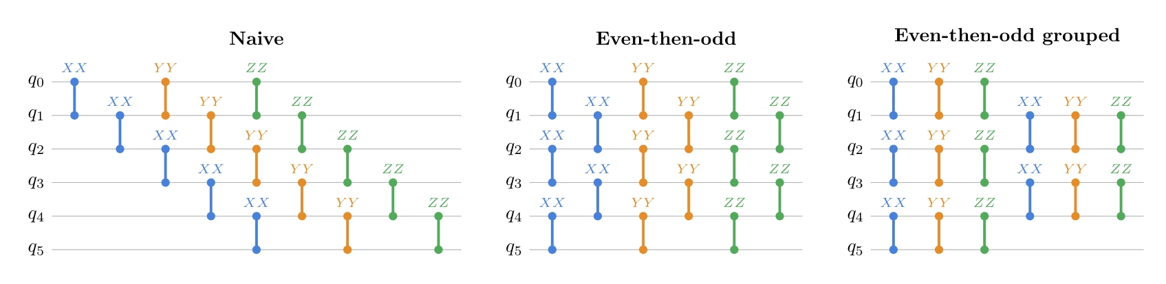
Pauli evolutions with different term ordering

A ordenação do Hamiltoniano também afeta o erro de Trotter. Se colocarmos termos que não comutam um ao lado do outro, as transições de base ocorrem com mais frequência, o que induz mais erro de Trotter. Ao agrupar termos que exigem a mesma transformação de base de Pauli, mudanças de base redundantes podem ser evitadas.

Aqui, a comparação usa o maior tempo de evolução que aparece nas estimativas de Krylov da primeira linha, $t_{\max} = (r-1)\Delta t,$ usando a mesma condição de transpilação.

Para medir o erro de Trotter, usamos a infidelidade do processo entre o circuito trotterizado e a evolução Hamiltoniana exata,

\begin{equation*} \text{Infidelity}(U,V) = 1-F(U,V) = 1 - \frac{|\operatorname{Tr}(U^\dagger V)|^2}{d^2}, \end{equation*}

where $d=2^n$ is the dimension of the Hilbert space.

Este diagnóstico usa matrizes densas, portanto é adequado para este pequeno exemplo de 12 qubits, mas não se destina a ser uma subrotina escalável.

# The comparison uses the largest time that appears in the first-row Krylov estimates.
# Circuit depth does not depend on this numeric value, but the Trotter error does.
comparison_time = (krylov_dim - 1) * dt

def make_heisenberg_hamiltonian_ordered(
    num_qubits: int,
    ordering: str,
    coupling: float = 1.0,
) -> SparsePauliOp:
    """Return the same Heisenberg Hamiltonian with a specified term ordering."""
    terms: list[tuple[str, complex]] = []
    even_edges = [(q, q + 1) for q in range(0, num_qubits - 1, 2)]
    odd_edges = [(q, q + 1) for q in range(1, num_qubits - 1, 2)]

    def append_term(q0: int, q1: int, pauli: str):
        label = ["I"] * num_qubits
        label[num_qubits - 1 - q0] = pauli[0]
        label[num_qubits - 1 - q1] = pauli[1]
        terms.append(("".join(label), coupling))

    if ordering == "naive":
        for pauli in ("XX", "YY", "ZZ"):
            for q in range(num_qubits - 1):
                append_term(q, q + 1, pauli)
    elif ordering == "even-then-odd":
        for pauli in ("XX", "YY", "ZZ"):
            for q0, q1 in even_edges + odd_edges:
                append_term(q0, q1, pauli)
    elif ordering == "even-odd edge-grouped":
        for q0, q1 in even_edges + odd_edges:
            for pauli in ("XX", "YY", "ZZ"):
                append_term(q0, q1, pauli)
    else:
        raise ValueError(f"Unknown ordering: {ordering}")

    return SparsePauliOp.from_list(terms).simplify()

def build_numeric_evolution_circuit(
    hamiltonian: SparsePauliOp,
    synthesis,
    time_value: float,
    **synthesis_kwargs,
) -> QuantumCircuit:
    """Build a numeric circuit for exp(-i H t) with a chosen synthesis rule."""
    evolution_gate = PauliEvolutionGate(
        hamiltonian,
        time=time_value,
        synthesis=synthesis(**synthesis_kwargs),
    )
    circuit = QuantumCircuit(hamiltonian.num_qubits)
    circuit.append(evolution_gate, range(hamiltonian.num_qubits))
    return circuit

def process_infidelity(
    circuit: QuantumCircuit,
    exact_matrix: np.ndarray,
) -> float:
    """Return 1 - |Tr(U_circuit† U_exact) / d|²."""
    circuit_matrix = np.asarray(Operator(circuit).data)
    dim = circuit_matrix.shape[0]
    normalized_trace = np.vdot(circuit_matrix, exact_matrix) / dim
    fidelity = np.abs(normalized_trace) ** 2
    return float(np.clip(1.0 - fidelity, 0.0, 1.0))

hamiltonians_by_ordering = {
    ordering: make_heisenberg_hamiltonian_ordered(
        num_qubits, ordering, coupling=1.0
    )
    for ordering in ["naive", "even-then-odd", "even-odd edge-grouped"]
}

print(f"Comparison time: {comparison_time}\n")

for order_name, ham_ordered in hamiltonians_by_ordering.items():
    print(f"{order_name}:")
    print([op for op, _ in ham_ordered.to_list()])
    print()

print("Precomputing the exact evolution operator... ", end="")
exact_matrix = la.expm(-1j * comparison_time * hamiltonian.to_matrix())
print("Done")

Comparison time: 0.8567979964335799

naive:
['IIIIIIIIIIXX', 'IIIIIIIIIXXI', 'IIIIIIIIXXII', 'IIIIIIIXXIII', 'IIIIIIXXIIII', 'IIIIIXXIIIII', 'IIIIXXIIIIII', 'IIIXXIIIIIII', 'IIXXIIIIIIII', 'IXXIIIIIIIII', 'XXIIIIIIIIII', 'IIIIIIIIIIYY', 'IIIIIIIIIYYI', 'IIIIIIIIYYII', 'IIIIIIIYYIII', 'IIIIIIYYIIII', 'IIIIIYYIIIII', 'IIIIYYIIIIII', 'IIIYYIIIIIII', 'IIYYIIIIIIII', 'IYYIIIIIIIII', 'YYIIIIIIIIII', 'IIIIIIIIIIZZ', 'IIIIIIIIIZZI', 'IIIIIIIIZZII', 'IIIIIIIZZIII', 'IIIIIIZZIIII', 'IIIIIZZIIIII', 'IIIIZZIIIIII', 'IIIZZIIIIIII', 'IIZZIIIIIIII', 'IZZIIIIIIIII', 'ZZIIIIIIIIII']

even-then-odd:
['IIIIIIIIIIXX', 'IIIIIIIIXXII', 'IIIIIIXXIIII', 'IIIIXXIIIIII', 'IIXXIIIIIIII', 'XXIIIIIIIIII', 'IIIIIIIIIXXI', 'IIIIIIIXXIII', 'IIIIIXXIIIII', 'IIIXXIIIIIII', 'IXXIIIIIIIII', 'IIIIIIIIIIYY', 'IIIIIIIIYYII', 'IIIIIIYYIIII', 'IIIIYYIIIIII', 'IIYYIIIIIIII', 'YYIIIIIIIIII', 'IIIIIIIIIYYI', 'IIIIIIIYYIII', 'IIIIIYYIIIII', 'IIIYYIIIIIII', 'IYYIIIIIIIII', 'IIIIIIIIIIZZ', 'IIIIIIIIZZII', 'IIIIIIZZIIII', 'IIIIZZIIIIII', 'IIZZIIIIIIII', 'ZZIIIIIIIIII', 'IIIIIIIIIZZI', 'IIIIIIIZZIII', 'IIIIIZZIIIII', 'IIIZZIIIIIII', 'IZZIIIIIIIII']

even-odd edge-grouped:
['IIIIIIIIIIXX', 'IIIIIIIIIIYY', 'IIIIIIIIIIZZ', 'IIIIIIIIXXII', 'IIIIIIIIYYII', 'IIIIIIIIZZII', 'IIIIIIXXIIII', 'IIIIIIYYIIII', 'IIIIIIZZIIII', 'IIIIXXIIIIII', 'IIIIYYIIIIII', 'IIIIZZIIIIII', 'IIXXIIIIIIII', 'IIYYIIIIIIII', 'IIZZIIIIIIII', 'XXIIIIIIIIII', 'YYIIIIIIIIII', 'ZZIIIIIIIIII', 'IIIIIIIIIXXI', 'IIIIIIIIIYYI', 'IIIIIIIIIZZI', 'IIIIIIIXXIII', 'IIIIIIIYYIII', 'IIIIIIIZZIII', 'IIIIIXXIIIII', 'IIIIIYYIIIII', 'IIIIIZZIIIII', 'IIIXXIIIIIII', 'IIIYYIIIIIII', 'IIIZZIIIIIII', 'IXXIIIIIIIII', 'IYYIIIIIIIII', 'IZZIIIIIIIII']

Precomputing the exact evolution operator... Done

Primeiro mantemos a regra de síntese fixa em um passo de Trotter de primeira ordem e variamos apenas a ordenação dos termos de Pauli. O objetivo desta comparação é principalmente ver o quanto a profundidade do circuito e o custo de dois qubits podem ser reduzidos ao expor arestas disjuntas de vizinhos mais próximos ao transpilador.

ordering_comparison_rows = []
infidelity_reps = [1, 2, 4, 8]

for ordering, ham_ordered in hamiltonians_by_ordering.items():
    for reps in infidelity_reps:
        circuit = build_numeric_evolution_circuit(
            ham_ordered,
            LieTrotter,
            comparison_time,
            reps=reps,
        )
        decomposed_circuit = simple_transpilation(circuit)
        infidelity = process_infidelity(decomposed_circuit, exact_matrix)
        ordering_comparison_rows.append(
            {
                "ordering": ordering,
                "synthesis": f"LieTrotter(reps={reps})",
                "infidelity": infidelity,
                **summarize_circuit(decomposed_circuit),
            }
        )
        if reps == 1:
            print(f"Circuit for {ordering} ordering:")
            print([op for op, _ in ham_ordered.to_list()])
            display(decomposed_circuit.draw("mpl", fold=-1, scale=0.6))

ordering_comparison_df = pd.DataFrame(ordering_comparison_rows)
display(ordering_comparison_df)

hamiltonian_for_synthesis = hamiltonians_by_ordering["even-odd edge-grouped"]

Circuit for naive ordering:
['IIIIIIIIIIXX', 'IIIIIIIIIXXI', 'IIIIIIIIXXII', 'IIIIIIIXXIII', 'IIIIIIXXIIII', 'IIIIIXXIIIII', 'IIIIXXIIIIII', 'IIIXXIIIIIII', 'IIXXIIIIIIII', 'IXXIIIIIIIII', 'XXIIIIIIIIII', 'IIIIIIIIIIYY', 'IIIIIIIIIYYI', 'IIIIIIIIYYII', 'IIIIIIIYYIII', 'IIIIIIYYIIII', 'IIIIIYYIIIII', 'IIIIYYIIIIII', 'IIIYYIIIIIII', 'IIYYIIIIIIII', 'IYYIIIIIIIII', 'YYIIIIIIIIII', 'IIIIIIIIIIZZ', 'IIIIIIIIIZZI', 'IIIIIIIIZZII', 'IIIIIIIZZIII', 'IIIIIIZZIIII', 'IIIIIZZIIIII', 'IIIIZZIIIIII', 'IIIZZIIIIIII', 'IIZZIIIIIIII', 'IZZIIIIIIIII', 'ZZIIIIIIIIII']

Output of the previous code cell

Circuit for even-then-odd ordering:
['IIIIIIIIIIXX', 'IIIIIIIIXXII', 'IIIIIIXXIIII', 'IIIIXXIIIIII', 'IIXXIIIIIIII', 'XXIIIIIIIIII', 'IIIIIIIIIXXI', 'IIIIIIIXXIII', 'IIIIIXXIIIII', 'IIIXXIIIIIII', 'IXXIIIIIIIII', 'IIIIIIIIIIYY', 'IIIIIIIIYYII', 'IIIIIIYYIIII', 'IIIIYYIIIIII', 'IIYYIIIIIIII', 'YYIIIIIIIIII', 'IIIIIIIIIYYI', 'IIIIIIIYYIII', 'IIIIIYYIIIII', 'IIIYYIIIIIII', 'IYYIIIIIIIII', 'IIIIIIIIIIZZ', 'IIIIIIIIZZII', 'IIIIIIZZIIII', 'IIIIZZIIIIII', 'IIZZIIIIIIII', 'ZZIIIIIIIIII', 'IIIIIIIIIZZI', 'IIIIIIIZZIII', 'IIIIIZZIIIII', 'IIIZZIIIIIII', 'IZZIIIIIIIII']

Output of the previous code cell

Circuit for even-odd edge-grouped ordering:
['IIIIIIIIIIXX', 'IIIIIIIIIIYY', 'IIIIIIIIIIZZ', 'IIIIIIIIXXII', 'IIIIIIIIYYII', 'IIIIIIIIZZII', 'IIIIIIXXIIII', 'IIIIIIYYIIII', 'IIIIIIZZIIII', 'IIIIXXIIIIII', 'IIIIYYIIIIII', 'IIIIZZIIIIII', 'IIXXIIIIIIII', 'IIYYIIIIIIII', 'IIZZIIIIIIII', 'XXIIIIIIIIII', 'YYIIIIIIIIII', 'ZZIIIIIIIIII', 'IIIIIIIIIXXI', 'IIIIIIIIIYYI', 'IIIIIIIIIZZI', 'IIIIIIIXXIII', 'IIIIIIIYYIII', 'IIIIIIIZZIII', 'IIIIIXXIIIII', 'IIIIIYYIIIII', 'IIIIIZZIIIII', 'IIIXXIIIIIII', 'IIIYYIIIIIII', 'IIIZZIIIIIII', 'IXXIIIIIIIII', 'IYYIIIIIIIII', 'IZZIIIIIIIII']

Output of the previous code cell

ordering           synthesis  infidelity  depth  size  \
                 naive  LieTrotter(reps=1)    0.999917     15    33   
                 naive  LieTrotter(reps=2)    0.805998     21    66   
                 naive  LieTrotter(reps=4)    0.271389     33   132   
                 naive  LieTrotter(reps=8)    0.074590     57   264   
         even-then-odd  LieTrotter(reps=1)    0.999917      6    33   
         even-then-odd  LieTrotter(reps=2)    0.805998     12    66   
         even-then-odd  LieTrotter(reps=4)    0.271389     24   132   
         even-then-odd  LieTrotter(reps=8)    0.074590     48   264   
 even-odd edge-grouped  LieTrotter(reps=1)    0.998432      6    33   
 even-odd edge-grouped  LieTrotter(reps=2)    0.653843     12    66   
even-odd edge-grouped  LieTrotter(reps=4)    0.181529     24   132   
even-odd edge-grouped  LieTrotter(reps=8)    0.045244     48   264   

    2q gates  2q depth  
       33        15  
       66        21  
      132        33  
      264        57  
       33         6  
       66        12  
      132        24  
      264        48  
       33         6  
       66        12  
     132        24  
     264        48

Em reps=1, observamos que tanto a ordenação par-depois-ímpar quanto a agrupada por aresta par-ímpar reduzem a profundidade de 15 para 6 ao expor camadas de dois qubits paralelas, enquanto a contagem de portas de dois qubits permanece a mesma nas três ordenações. No entanto, as três ordenações têm infidelidade próxima de 1, então variamos o número de repetições de Trotter para separar as ordenações de forma mais clara. À medida que o número de repetições aumenta, a infidelidade da ordenação even-odd edge-grouped cai mais rápido do que as outras duas, atingindo 0,045 em reps=8 contra 0,075 para a ordenação ingênua e a par-depois-ímpar.

Comparar a síntese de fórmula de produto

Em seguida, exploramos diferentes configurações avançadas de trotterização, com a ordenação Hamiltoniana fixa na ordenação agrupada por aresta par-ímpar. Consideramos Lie-Trotter de primeira ordem, Suzuki-Trotter de segunda ordem e Suzuki-Trotter de quarta ordem.

synthesis_comparison_rows = []

for num_trotter_steps in [1, 2, 3, 4, 5]:
    synthesis_cases = [
        ("LieTrotter", LieTrotter, {"reps": num_trotter_steps}),
        (
            "SuzukiTrotter(order=2)",
            SuzukiTrotter,
            {"order": 2, "reps": num_trotter_steps},
        ),
        (
            "SuzukiTrotter(order=4)",
            SuzukiTrotter,
            {"order": 4, "reps": num_trotter_steps},
        ),
    ]
    for label, synthesis, kwargs in synthesis_cases:
        circuit = build_numeric_evolution_circuit(
            hamiltonian_for_synthesis,
            synthesis,
            comparison_time,
            **kwargs,
        )
        decomposed_circuit = simple_transpilation(circuit)
        synthesis_comparison_rows.append(
            {
                "synthesis": label,
                "reps": kwargs["reps"],
                "infidelity": process_infidelity(
                    decomposed_circuit, exact_matrix
                ),
                **summarize_circuit(decomposed_circuit),
            }
        )

synthesis_comparison_df = pd.DataFrame(synthesis_comparison_rows)
display(synthesis_comparison_df.sort_values(["2q gates", "2q depth"]))

# For memory free
exact_matrix = None

synthesis  reps    infidelity  depth  size  2q gates  \
             LieTrotter     1  9.984324e-01      6    33        33   
 SuzukiTrotter(order=2)     1  9.733399e-01      9    51        51   
             LieTrotter     2  6.538427e-01     12    66        66   
 SuzukiTrotter(order=2)     2  2.522533e-01     15    84        84   
             LieTrotter     3  3.197242e-01     18    99        99   
 SuzukiTrotter(order=2)     3  4.804050e-02     21   117       117   
             LieTrotter     4  1.815291e-01     24   132       132   
SuzukiTrotter(order=2)     4  1.453103e-02     27   150       150   
            LieTrotter     5  1.161770e-01     30   165       165   
 SuzukiTrotter(order=4)     1  2.884402e-01     33   183       183   
SuzukiTrotter(order=2)     5  5.803455e-03     33   183       183   
 SuzukiTrotter(order=4)     2  1.641162e-03     63   348       348   
 SuzukiTrotter(order=4)     3  2.907076e-05     93   513       513   
SuzukiTrotter(order=4)     4  2.791061e-06    123   678       678   
SuzukiTrotter(order=4)     5  4.736685e-07    153   843       843   

    2q depth  
        6  
        9  
       12  
       15  
       18  
       21  
       24  
      27  
      30  
       33  
      33  
       63  
       93  
     123  
     153

O Lie-Trotter fornece o circuito mais raso, mas tem o maior erro, enquanto o Suzuki-Trotter de quarta ordem é mais preciso, mas aumenta a profundidade do circuito. Para o restante do tutorial, escolhemos o Suzuki-Trotter de segunda ordem porque ele fornece um circuito de pequena profundidade enquanto reduz substancialmente o erro de Trotter em relação à fórmula de primeira ordem.

Remover a porta de evolução temporal controlada

No teste de troca estendido, controlar a evolução temporal com um único qubit ancilla exige que o ancilla controle muitas portas em todo o sistema. Isso pode introduzir uma sobrecarga substancial de roteamento e, no pior caso, exige efetivamente conectividade de todos para um. Para evitar isso, é possível uma otimização adicional substituindo a porta de evolução temporal controlada por uma versão livre de controle, explorando a simetria do Hamiltoniano. Vamos observar o seguinte circuito.

circuit optimization

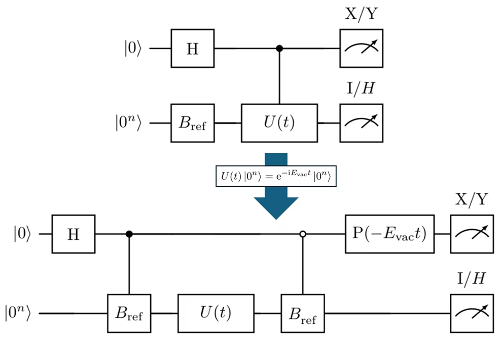
Aqui, $B_{\rm ref}$ prepara o estado de referência, $B_{\rm ref}|0^n\rangle = |\psi_{0}\rangle$ .

Em vez de primeiro preparar $\frac{1}{\sqrt{2}}(|0\rangle+|1\rangle)|\psi_0\rangle$ e depois aplicar $U(t)$ apenas no ramo $|1\rangle$ , o circuito prepara diretamente os dois ramos como

\begin{equation*} |0\rangle|\psi_0\rangle \quad \text{and} \quad |1\rangle|\psi_d\rangle , \end{equation*}

where

\begin{equation*} |\psi_d\rangle = U(d\Delta t)|\psi_0\rangle . \end{equation*}

O circuito primeiro aplica uma porta Hadamard ao ancilla e prepara o estado de referência apenas no ramo $|1\rangle$ :

\begin{equation*} |0\rangle |0^n\rangle \longrightarrow \frac{|0\rangle |0^n\rangle + |1\rangle B_{\rm ref}|0^n\rangle}{\sqrt{2}} = \frac{|0\rangle |0^n\rangle + |1\rangle |\psi_0\rangle}{\sqrt{2}} . \end{equation*}

Em seguida, o operador de evolução temporal não controlado é aplicado a ambos os ramos:

\begin{equation*} \frac{|0\rangle |0^n\rangle + |1\rangle |\psi_0\rangle}{\sqrt{2}} \longrightarrow \frac{|0\rangle U(t)|0^n\rangle + |1\rangle U(t)|\psi_0\rangle}{\sqrt{2}} . \end{equation*}

Como o Hamiltoniano preserva o número de excitações, podemos ver que $|0^n\rangle$ é seu autoestado, e portanto o operador de evolução acumula apenas uma fase sob o Hamiltoniano:

\begin{equation*} U(t)|0^n\rangle = e^{-iE_{\rm vac}t}|0^n\rangle . \end{equation*}

Therefore,

\begin{equation*} \frac{|0\rangle U(t)|0^n\rangle + |1\rangle U(t)|\psi_0\rangle}{\sqrt{2}} = \frac{e^{-iE_{\rm vac}t}|0\rangle |0^n\rangle + |1\rangle U(t)|\psi_0\rangle}{\sqrt{2}} . \end{equation*}

Em seguida, $B_{\rm ref}$ é aplicado apenas no ramo $|0\rangle$ .

\begin{equation*} \frac{e^{-iE_{\rm vac}t}|0\rangle |\psi_0\rangle + |1\rangle U(t)|\psi_0\rangle}{\sqrt{2}} . \end{equation*}

Neste ponto, os dois ramos têm uma fase relativa extra. Para removê-la, aplicamos a porta de fase do ancilla

\begin{equation*} P(-E_{\rm vac}t) = \begin{pmatrix} 1 & 0 \\ 0 & e^{-iE_{\rm vac}t} \end{pmatrix}. \end{equation*}

Isso transforma o estado como

\begin{equation*} \frac{e^{-iE_{\rm vac}t}|0\rangle |\psi_0\rangle + |1\rangle U(t)|\psi_0\rangle}{\sqrt{2}} \longrightarrow \frac{e^{-iE_{\rm vac}t}|0\rangle |\psi_0\rangle + e^{-iE_{\rm vac}t}|1\rangle U(t)|\psi_0\rangle}{\sqrt{2}} . \end{equation*}

Assim, a menos de uma fase global irrelevante, finalmente preparamos

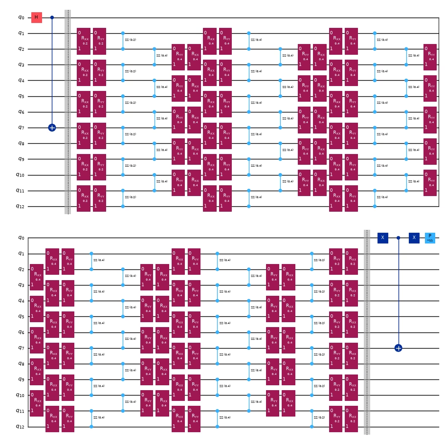
\begin{equation*} |\Phi_{0d}\rangle = \frac{ |0\rangle|\psi_0\rangle + |1\rangle U(t)|\psi_0\rangle }{\sqrt{2}} . \end{equation*}

No próximo bloco de código, implementamos este circuito livre de controle.

controlled_extended_swap_test = extended_swap_test

# Reuse the ordering and synthesis rule selected by the comparison above.
evol_gate_optimized = PauliEvolutionGate(
    hamiltonian_for_synthesis,
    time=t,
    synthesis=SuzukiTrotter(order=2, reps=num_trotter_steps),
)

uncontrolled_evolution = QuantumCircuit(num_qubits, name="U_ST2(t)")
uncontrolled_evolution.append(evol_gate_optimized, range(num_qubits))

controlled_state_prep = QuantumCircuit(num_qubits + 1, name="C-Prep")
for q, bit in enumerate(reversed(ref_bitstring)):
    if bit == "1":
        controlled_state_prep.cx(ancilla, system_qubits[q])

vacuum_bitstring = "0" * num_qubits
vacuum_energy = basis_state_expectation_sparse(hamiltonian, "0" * num_qubits)

optimized_extended_swap_test = QuantumCircuit(num_qubits + 1)
optimized_extended_swap_test.h(ancilla)

# Prepare |psi_ref> only on the |1> branch.
optimized_extended_swap_test.compose(controlled_state_prep, inplace=True)
optimized_extended_swap_test.barrier()

# Apply the Trotterized time evolution without control.
optimized_extended_swap_test.compose(
    uncontrolled_evolution,
    qubits=system_qubits,
    inplace=True,
)
optimized_extended_swap_test.barrier()

# Map |0>|0...0> to |0>|psi_ref>, leaving the |1> branch unchanged.
optimized_extended_swap_test.x(ancilla)
optimized_extended_swap_test.compose(controlled_state_prep, inplace=True)
optimized_extended_swap_test.x(ancilla)

# Cancel the known vacuum phase so that the same X/Y observables can be used.
optimized_extended_swap_test.p(-vacuum_energy * t, ancilla)
optimized_extended_swap_test = simple_transpilation(
    optimized_extended_swap_test
)

print(f"Vacuum energy E_vac = {vacuum_energy:.1f}")
display(
    optimized_extended_swap_test.assign_parameters({t: 1.0}).draw(
        "mpl", scale=0.5, fold=26
    )
)

Vacuum energy E_vac = 11.0+0.0j

Output of the previous code cell

Transpilação

Agora, transpilamos os circuitos controlado e livre de controle para que se tornem executáveis no hardware. Vamos comparar o resultado dos circuitos transpilados.

pass_manager = generate_preset_pass_manager(
    backend=backend,
    optimization_level=3,
)

isa_controlled_extended_swap_test = pass_manager.run(
    controlled_extended_swap_test
)

pass_manager = generate_preset_pass_manager(
    backend=backend, optimization_level=3, routing_method="none"
)
isa_optimized_extended_swap_test = pass_manager.run(
    optimized_extended_swap_test
)

transpilation_result = [
    {
        "label": "abstract controlled U(t)",
        **summarize_circuit(isa_controlled_extended_swap_test),
    },
    {
        "label": "optimized non-controlled U(t)",
        **summarize_circuit(isa_optimized_extended_swap_test),
    },
]

display(pd.DataFrame(transpilation_result))

def filter_qubits_from_layout(layout):
    q_layout = Layout(
        {
            physical: virtual
            for physical, virtual in layout.get_physical_bits().items()
            if virtual._register.name == "q"
        }
    )
    return q_layout

print(
    filter_qubits_from_layout(
        isa_optimized_extended_swap_test.layout.initial_layout
    )
)

isa_observables = [
    op.apply_layout(isa_optimized_extended_swap_test.layout)
    for op in observables
]

label  depth   size  2q gates  2q depth
0       abstract controlled U(t)  15457  23786      4686      4580
1  optimized non-controlled U(t)    261   1716       307        57

Layout({
<Qubit register=(13, "q"), index=0>,
<Qubit register=(13, "q"), index=1>,
<Qubit register=(13, "q"), index=2>,
<Qubit register=(13, "q"), index=3>,
<Qubit register=(13, "q"), index=4>,
<Qubit register=(13, "q"), index=5>,
<Qubit register=(13, "q"), index=6>,
<Qubit register=(13, "q"), index=7>,
<Qubit register=(13, "q"), index=8>,
<Qubit register=(13, "q"), index=9>,
<Qubit register=(13, "q"), index=10>,
<Qubit register=(13, "q"), index=11>,
<Qubit register=(13, "q"), index=12>
})

Etapa 3: Executar usando primitivas do Qiskit

O próximo passo é submeter o mesmo circuito parametrizado para vários valores de $d$ . Para cada $d$ , estimamos quatro valores esperados: $X\otimes I$ , $Y\otimes I$ , $X\otimes (H-T)$ , e $Y\otimes (H-T)$ . Esses quatro números são então combinados nos elementos complexos da primeira linha $\mathcal{S}_{0d}$ e $\mathcal{H}_{0d}$ .

Aqui, $\mathcal{S}_{00}=1$ e $\mathcal{H}_{00}=\langle\psi_{0}|(H-T)|\psi_{0}\rangle=\langle\psi_{0}|H|\psi_{0}\rangle-\tau$ podem ser calculados classicamente, já que $\lvert\psi_0\rangle$ é esparso, então pulamos o caso $d=0$ .

pub_list = []
d_values = list(range(1, krylov_dim))

# Exact local statevector estimator.
estimator = StatevectorEstimator()

# We use the circuit before the transpilation for the local simulator,
# but we will use the transpiled circuit for the real backend.
for d in d_values:
    parameter_values = [d * dt]

    for ob in observables:
        pub_list.append(
            (
                optimized_extended_swap_test,
                ob,
                parameter_values,
            )
        )

job = estimator.run(pub_list)

# Local PrimitiveJob does not provide Runtime-style job inputs,
# so preserve the inputs directly.
inputs = pub_list
result = job.result()

print(f"Number of Krylov basis states: r = {len(d_values)}")
print(f"Number of PUBs: {len(pub_list)}")
print(f"Each d uses observables: {observable_labels}")

Number of Krylov basis states: r = 9
Number of PUBs: 36
Each d uses observables: ['Re S_0d', 'Im S_0d', 'Re shifted H_0d', 'Im shifted H_0d']

Etapa 4: Pós-processar e retornar o resultado no formato clássico desejado

Depois de estimar as matrizes projetadas, regularizamos e resolvemos o GEVP

\begin{equation*} \mathcal{H}\mathbf{c} = E\mathcal{S}\mathbf{c}. \end{equation*}

O menor autovalor generalizado fornece a estimativa KQD da energia do estado fundamental.

h_shifted_row_est = np.zeros(krylov_dim, dtype=complex)
s_row_est = np.zeros(krylov_dim, dtype=complex)

h_shifted_row_est[0] = ref_energy - shift_tau
s_row_est[0] = 1.0

for idx, (pub_input, pub_result) in enumerate(zip(inputs, result)):
    d_index, obs_index = divmod(idx, len(observables))
    ev = np.asarray(pub_result.data.evs).reshape(-1)[0]
    std = np.asarray(pub_result.data.stds).reshape(-1)[0]

    if obs_index == 0:
        s_row_est[d_index + 1] = ev
    elif obs_index == 1:
        s_row_est[d_index + 1] += 1j * ev
    elif obs_index == 2:
        h_shifted_row_est[d_index + 1] = ev
    elif obs_index == 3:
        h_shifted_row_est[d_index + 1] += 1j * ev

# H_0d = shifted_H_0d + tau * S_0d.
h_row_est = h_shifted_row_est + shift_tau * s_row_est

h_matrix_est = la.toeplitz(h_row_est.conj(), h_row_est)
s_matrix_est = la.toeplitz(s_row_est.conj(), s_row_est)

s_eigvals = la.eigvalsh(0.5 * (s_matrix_est + s_matrix_est.conj().T))
positive_s_eigvals = s_eigvals[s_eigvals > 1e-12]
s_condition_number = (
    positive_s_eigvals[-1] / positive_s_eigvals[0]
    if len(positive_s_eigvals) > 0
    else np.inf
)

with np.printoptions(precision=3, suppress=True):
    print("Estimated first row of S:")
    print(s_row_est)
    print()
    print("Estimated first row of H:")
    print(h_row_est)
    print()
    print("Eigenvalues of the estimated overlap matrix S:")
    print(s_eigvals)
    print(f"Condition number above 1e-12: {s_condition_number:.3e}")
    print()

Estimated first row of S:
[ 1.   +0.j     0.758-0.596j  0.203-0.836j -0.291-0.636j -0.444-0.229j
 -0.276+0.053j -0.044+0.051j  0.006-0.121j -0.155-0.218j -0.345-0.101j]

Estimated first row of H:
[ 7.   +0.j     4.842-4.76j   0.044-6.185j -3.791-3.653j -4.137+0.39j
 -1.495+2.654j  1.331+1.777j  1.85 -0.763j -0.032-2.278j -2.222-1.372j]

Eigenvalues of the estimated overlap matrix S:
[-0.     0.     0.     0.     0.     0.     0.01   0.355  3.526  6.109]
Condition number above 1e-12: 1.904e+12

Agora resolvemos o problema de autovalor generalizado usando as matrizes reconstruídas a partir das estimativas do circuito. Em um cálculo ideal de vetor de estado com evolução exata em tempo real, isso deve reproduzir o resultado projetado exato. Na prática, os desvios podem vir da trotterização, do erro de amostragem e da instabilidade numérica da matriz de sobreposição.

Observamos como a energia converge à medida que aumentamos a dimensão do subespaço de Krylov.

exact_evals = diagonalize_single_1_subspace(hamiltonian)
exact_ground = min(exact_evals)
print("exact ground state energy:  ", exact_ground)

threshold = 1e-12
energy_convergence = []

for r in range(1, krylov_dim + 1):
    energy_est_kqd, coeffs_est, retained_est = solve_thresholded_gevp(
        h_matrix_est[:r, :r],
        s_matrix_est[:r, :r],
        threshold=threshold,
    )
    energy_convergence.append(energy_est_kqd)
    print(
        f"Krylov ground state energy (dim={r}, retained={retained_est}): ",
        energy_est_kqd,
    )

exact ground state energy:   3.136296694843727
Krylov ground state energy (dim=1, retained=1):  7.0
Krylov ground state energy (dim=2, retained=2):  4.184510657551266
Krylov ground state energy (dim=3, retained=3):  3.5539074630394136
Krylov ground state energy (dim=4, retained=4):  3.3366270761341044
Krylov ground state energy (dim=5, retained=5):  3.252017453225087
Krylov ground state energy (dim=6, retained=6):  3.2300275138879186
Krylov ground state energy (dim=7, retained=7):  3.2299154099085685
Krylov ground state energy (dim=8, retained=7):  3.2298063744216776
Krylov ground state energy (dim=9, retained=7):  3.2296778282872456
Krylov ground state energy (dim=10, retained=8):  3.223647515867734

def plot_energy_convergence(energy_convergence, exact_ground, krylov_dim):
    fig, ax = plt.subplots(figsize=(7, 4.5))

    ax.plot(
        range(1, krylov_dim + 1),
        energy_convergence,
        marker="o",
        label="KQD estimate",
    )

    ax.axhline(
        exact_ground,
        linestyle="--",
        label=f"Exact ground energy = {exact_ground:.6f}",
    )

    ax.set_xlabel("Krylov dimension")
    ax.set_ylabel("Ground-state energy")
    ax.grid(True, alpha=0.3)
    ax.legend()
    plt.tight_layout()
    plt.show()

plot_energy_convergence(energy_convergence, exact_ground, krylov_dim)

Output of the previous code cell

Exemplo de hardware em larga escala

A seção anterior usou um modelo de 12 qubits para que a simulação de vetor de estado pudesse ser usada como diagnóstico. Agora escalamos o mesmo fluxo de trabalho KQD para uma cadeia de Heisenberg de 30 qubits e preparamos a carga de trabalho para execução em hardware do IBM Quantum.

Passos 1-4 comprimidos em um único bloco de código

Aqui agora juntamos todos esses detalhes em um único fluxo de trabalho em uma escala maior, que é então executado em nosso hardware quântico real. Nesta seção, aplicamos configurações realistas de mitigação de erros para melhorar a confiabilidade dos resultados. Como os elementos de matriz correspondentes a diferentes valores de $d$ podem ser avaliados em paralelo, usamos o modo Batch para executá-los de forma eficiente.

# -------------------------Step 1-------------------------

# Map the classical problem to quantum circuits and observables.
# Problem and KQD parameters.
large_num_qubits = 30
large_krylov_dim = 7
large_num_trotter_steps = 3
large_dt = np.pi / (3 * (large_num_qubits - 1))
large_t = Parameter("t_large")

# Use a single excitation near the center of the chain.
large_excitation_qubit = large_num_qubits // 2
large_ref_label = ["0"] * large_num_qubits
large_ref_label[large_num_qubits - 1 - large_excitation_qubit] = "1"
large_ref_bitstring = "".join(large_ref_label)

# Use the ordering and product formula selected in the preceding section.
large_hamiltonian = make_heisenberg_hamiltonian_ordered(
    large_num_qubits,
    ordering="even-odd edge-grouped",
    coupling=1.0,
)
large_ref_energy = float(
    np.real(
        basis_state_expectation_sparse(large_hamiltonian, large_ref_bitstring)
    )
)
large_vacuum_energy = float(
    np.real(
        basis_state_expectation_sparse(
            large_hamiltonian, "0" * large_num_qubits
        )
    )
)

large_evolution_gate = PauliEvolutionGate(
    large_hamiltonian,
    time=large_t,
    synthesis=SuzukiTrotter(order=2, reps=large_num_trotter_steps),
)
large_uncontrolled_evolution = QuantumCircuit(
    large_num_qubits,
    name="U_ST2_large(t)",
)
large_uncontrolled_evolution.append(
    large_evolution_gate,
    range(large_num_qubits),
)

# Build the control-free extended-swap-test circuit.
large_ancilla = 0
large_system_qubits = list(range(1, large_num_qubits + 1))

large_controlled_state_prep = QuantumCircuit(
    large_num_qubits + 1,
    name="C-Prep-large",
)
large_controlled_state_prep.cx(
    large_ancilla,
    large_system_qubits[large_excitation_qubit],
)

large_extended_swap_test = QuantumCircuit(large_num_qubits + 1)
large_extended_swap_test.h(large_ancilla)
large_extended_swap_test.compose(large_controlled_state_prep, inplace=True)
large_extended_swap_test.compose(
    large_uncontrolled_evolution,
    qubits=large_system_qubits,
    inplace=True,
)
large_extended_swap_test.x(large_ancilla)
large_extended_swap_test.compose(
    large_controlled_state_prep.inverse(),
    inplace=True,
)
large_extended_swap_test.x(large_ancilla)
large_extended_swap_test.p(
    -large_vacuum_energy * large_t,
    large_ancilla,
)

# Reuse the Hamiltonian-shifting construction from the preceding section.
(
    large_obs_x_shifted_hamiltonian,
    large_obs_y_shifted_hamiltonian,
    large_shift_tau,
) = make_reduced_heisenberg_observables(large_ref_bitstring)

large_observables = [
    SparsePauliOp("I" * large_num_qubits + "X"),
    SparsePauliOp("I" * large_num_qubits + "Y"),
    large_obs_x_shifted_hamiltonian,
    large_obs_y_shifted_hamiltonian,
]
large_observable_labels = [
    "Re S_0d",
    "Im S_0d",
    "Re shifted H_0d",
    "Im shifted H_0d",
]

# -------------------------Step 2-------------------------

# Optimize the problem for quantum execution.
# Select a real backend and transpile the parameterized circuit to ISA form.
large_backend = service.backend("ibm_boston")
large_pass_manager = generate_preset_pass_manager(
    backend=large_backend, optimization_level=3, routing_method="none"
)
large_isa_circuit = large_pass_manager.run(large_extended_swap_test)
large_isa_observables = [
    observable.apply_layout(large_isa_circuit.layout)
    for observable in large_observables
]

large_two_qubit_gate_count = sum(
    instruction.operation.num_qubits == 2
    for instruction in large_isa_circuit.data
)

print(f"Backend: {large_backend.name}")
print(f"System qubits: {large_num_qubits}")
print(f"Total circuit qubits: {large_isa_circuit.num_qubits}")
print(f"Krylov dimension: {large_krylov_dim}")
print(f"Time step: {large_dt:.6f}")
print(f"Shift tau: {large_shift_tau}")
print(f"ISA circuit depth: {large_isa_circuit.depth()}")
print(f"ISA two-qubit gates: {large_two_qubit_gate_count}")
print(
    f"ISA two-qubit depth: {large_isa_circuit.depth(lambda x: x[0].num_qubits == 2)}"
)

# -------------------------Step 3-------------------------

# Execute on quantum hardware with Qiskit Runtime primitives.
# Submit one job per d, with all four observables in that job.
large_d_values = list(range(1, large_krylov_dim))
retrieve_batch_id = None
large_jobs = []

if retrieve_batch_id is None:
    large_estimator_options = {
        "default_shots": 8192,
        "dynamical_decoupling": {
            "enable": True,
            "sequence_type": "XpXm",
        },
        "resilience": {
            "measure_mitigation": True,
            "measure_noise_learning": {
                "num_randomizations": 32,
                "shots_per_randomization": 256,
            },
            "layer_noise_learning": {
                "max_layers_to_learn": 4,
                "layer_pair_depths": [0, 1, 2, 4, 16, 32],
                "num_randomizations": 32,
                "shots_per_randomization": 128,
            },
            "zne_mitigation": True,
            "zne": {
                "amplifier": "pea",
                "noise_factors": [1.0, 1.5, 2.0],
                "extrapolator": ("exponential", "linear"),
            },
        },
        "twirling": {
            "enable_gates": True,
            "enable_measure": True,
            "num_randomizations": 32,
            "shots_per_randomization": 256,
            "strategy": "active-accum",
        },
    }

    with Batch(backend=large_backend) as large_batch:
        large_batch_id = large_batch.session_id
        large_estimator = EstimatorV2(
            mode=large_batch,
            options=large_estimator_options,
        )
        # Krylov quantum diagonalization of lattice Hamiltonians -> TUT_KQDOLH.
        large_estimator.options.environment.job_tags = ["TUT_KQDOLH"]

        for d in large_d_values:
            parameter_values = [d * large_dt]
            pubs_for_d = [
                (large_isa_circuit, observable, parameter_values)
                for observable in large_isa_observables
            ]
            job = large_estimator.run(pubs_for_d)
            large_jobs.append(job)
            print(
                f"Submitted d={d}: job_id={job.job_id()}, "
                f"PUBs={len(pubs_for_d)}"
            )

    print(f"Batch ID: {large_batch_id}")
else:
    large_batch_id = retrieve_batch_id
    large_jobs = service.jobs(
        session_id=large_batch_id,
        limit=None,
        descending=False,
    )

large_job_ids_by_d = {
    d: job.job_id() for d, job in zip(large_d_values, large_jobs)
}
print(f"Job IDs by d: {large_job_ids_by_d}")

# -------------------------Step 4-------------------------

# Post-process the quantum results and solve the classical GEVP.
# Reconstruct the first rows of S and the shifted Hamiltonian matrix.
large_s_row_est = np.zeros(large_krylov_dim, dtype=complex)
large_h_shifted_row_est = np.zeros(large_krylov_dim, dtype=complex)
large_s_row_est[0] = 1.0
large_h_shifted_row_est[0] = large_ref_energy - large_shift_tau

for d, job in zip(large_d_values, large_jobs):
    job_result = job.result()

    if len(job_result) != len(large_observables):
        raise RuntimeError(
            f"Expected {len(large_observables)} PUB results for d={d}, "
            f"but received {len(job_result)}."
        )

    expectation_values = [
        np.asarray(pub_result.data.evs).reshape(-1)[0]
        for pub_result in job_result
    ]

    large_s_row_est[d] = expectation_values[0] + 1j * expectation_values[1]
    large_h_shifted_row_est[d] = (
        expectation_values[2] + 1j * expectation_values[3]
    )

# H_0d = shifted_H_0d + tau * S_0d.
large_h_row_est = large_h_shifted_row_est + large_shift_tau * large_s_row_est

large_s_matrix_est = la.toeplitz(
    large_s_row_est.conj(),
    large_s_row_est,
)
large_h_matrix_est = la.toeplitz(
    large_h_row_est.conj(),
    large_h_row_est,
)

large_exact_gnd = min(diagonalize_single_1_subspace(large_hamiltonian))

large_energy_convergence = []

with np.printoptions(precision=5, suppress=True):
    print("Estimated first row of S:")
    print(large_s_row_est)
    print("Estimated first row of H:")
    print(large_h_row_est)
    print("exact ground state energy:  ", large_exact_gnd)

    for r in range(1, large_krylov_dim + 1):
        energy_est_kqd, coeffs_est, retained_est = solve_thresholded_gevp(
            large_h_matrix_est[:r, :r],
            large_s_matrix_est[:r, :r],
            threshold=5e-2,
        )
        large_energy_convergence.append(energy_est_kqd)
        print(
            f"Krylov ground state energy (dim={r}, retained={retained_est}): ",
            energy_est_kqd,
        )

plot_energy_convergence(
    large_energy_convergence, large_exact_gnd, large_krylov_dim
)

Backend: ibm_boston
System qubits: 30
Total circuit qubits: 156
Krylov dimension: 7
Time step: 0.036110
Shift tau: 25.0
ISA circuit depth: 219
ISA two-qubit gates: 728
ISA two-qubit depth: 52
Job IDs by d: {1: 'd9fl4p4jeosc73fk4dg0', 2: 'd9fl4pineu4c739poecg', 3: 'd9fl4q2neu4c739poedg', 4: 'd9fl4qhhtsac739fjgn0', 5: 'd9fl4r4jeosc73fk4dhg', 6: 'd9fl4rkjeosc73fk4dj0'}
Estimated first row of S:
[ 1.     +0.j       0.42055-0.65466j -0.17883-0.73125j -0.64523-0.31601j
 -0.70781+0.55574j -0.02467+0.70525j  0.59301+0.55602j]
Estimated first row of H:
[ 25.      +0.j       10.3419 -16.5586j   -5.017  -18.03933j
 -16.44797 -6.98173j -17.17081+14.84502j   0.62722+17.81196j
  15.68886+12.74875j]
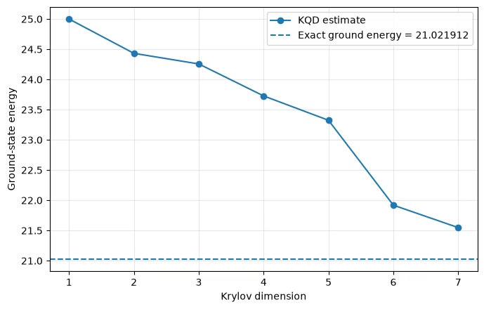
exact ground state energy:   21.021912418526902
Krylov ground state energy (dim=1, retained=1):  25.0
Krylov ground state energy (dim=2, retained=2):  24.432409110686205
Krylov ground state energy (dim=3, retained=3):  24.256856893278556
Krylov ground state energy (dim=4, retained=4):  23.727409826799715
Krylov ground state energy (dim=5, retained=4):  23.324720470780864
Krylov ground state energy (dim=6, retained=5):  21.91957579005085
Krylov ground state energy (dim=7, retained=5):  21.548331214122644

Output of the previous code cell

Apêndice: A perspectiva da função hamiltoniana (filtro espectral)

O fluxo de trabalho principal apresentou a KQD de forma operacional: construir uma base de Krylov a partir de estados evoluídos em tempo real, estimar as matrizes projetadas $\mathcal{H}$ e $\mathcal{S}$ , e resolver o GEVP. Este apêndice revisita a mesma computação a partir de um ângulo complementar que explica por que a KQD funciona: a perspectiva da função hamiltoniana, ou filtro espectral [3], [5]. Ele reutiliza o modelo de 12 qubits, o passo de tempo $\Delta t$ , e a solução de Krylov já obtida acima; nenhuma nova execução de circuito é necessária.

O estado de referência como uma distribuição de energia

Seja a decomposição espectral do hamiltoniano

\begin{equation*} H=\sum_{m} E_m\,|E_m\rangle\!\langle E_m|, \qquad E_0\le E_1\le\cdots, \end{equation*}

com autoestados de energia $|E_m\rangle$ . Qualquer estado de referência pode ser expandido nesta autobase,

\begin{equation*} |\psi_{0}\rangle=\sum_m a_m\,|E_m\rangle, \qquad a_m=\langle E_m|\psi_{0}\rangle, \end{equation*}

então carrega um peso espectral $p_m=|a_m|^2$ em cada energia $E_m$ . A energia de referência é a média desta distribuição, $\langle H\rangle_{0}=\sum_m p_m E_m$ .

A decomposição espectral de um Hamiltoniano geral de $n$ qubits tem custo exponencial, então essa visão serve apenas como diagnóstico e não faz parte do algoritmo. Aqui, no entanto, podemos calculá-la de forma barata para o mesmo problema com $n=12$ : o Hamiltoniano de Heisenberg conserva o número total de excitações, e a referência $|000001000000\rangle$ carrega uma única excitação, então todo o seu conteúdo espectral vive no subespaço de excitação única, cuja dimensão cresce apenas linearmente com $n$ . Portanto, reutilizamos o bloco exato de excitação única (já usado acima como benchmark) e extraímos a distribuição de referência $\{(E_m, p_m)\}$ dentro desse subespaço.

# Exact single-excitation-subspace decomposition of the reference state.
# This reuses make_heisenberg_hamiltonian / _basis_state_transition_amplitude_sparse
# and the n=12 `hamiltonian` and `ref_bitstring` defined in the small-scale example.
single_excitation_states = [1 << k for k in range(num_qubits)]

h_single = np.array(
    [
        [
            _basis_state_transition_amplitude_sparse(hamiltonian, bra, ket)
            for ket in single_excitation_states
        ]
        for bra in single_excitation_states
    ]
)
h_single = 0.5 * (h_single + h_single.conj().T)

subspace_evals, subspace_evecs = la.eigh(h_single)
subspace_evals = np.real(subspace_evals)

# Reference-state coordinates inside the single-excitation subspace.
ref_position = single_excitation_states.index(int(ref_bitstring, 2))
ref_in_subspace = np.zeros(num_qubits, dtype=complex)
ref_in_subspace[ref_position] = 1.0

# Amplitudes and spectral weights of the reference in the energy eigenbasis.
ref_eigen_amplitudes = subspace_evecs.conj().T @ ref_in_subspace
ref_spectral_weights = np.abs(ref_eigen_amplitudes) ** 2

print(f"Single-excitation subspace dimension: {num_qubits}")
print(f"Subspace ground-state energy:         {subspace_evals[0]:.6f}")
print(
    f"Reference energy (sum p_m E_m):       {np.sum(ref_spectral_weights * subspace_evals):.6f}"
)
print(f"Reference weight on subspace ground:  {ref_spectral_weights[0]:.6f}")

Single-excitation subspace dimension: 12
Subspace ground-state energy:         3.136297
Reference energy (sum p_m E_m):       7.000000
Reference weight on subspace ground:  0.163827

O KQD aprende um filtro que remodela esta distribuição

Uma função hamiltoniana $f(H)$ é definida por meio do cálculo espectral,

\begin{equation*} f(H)=\sum_m f(E_m)\,|E_m\rangle\!\langle E_m|, \end{equation*}

ou, em outras palavras, uma soma ponderada de autoprojetores. Aplicá-la à referência remodela cada amplitude espectral, $a_m \to a_m f(E_m)$ :

\begin{equation*} f(H)\,|\psi_{0}\rangle=\sum_m a_m\,f(E_m)\,|E_m\rangle . \end{equation*}

Se $f$ fosse fortemente concentrada na energia mais baixa ( $f(E_0)=1$ e $f(E_m)\approx 0$ caso contrário), então $f(H)$ atuaria como um projetor do estado fundamental, e a saída normalizada seria (próxima) ao estado fundamental. Portanto, um bom filtro espectral passa-baixa em energia é exatamente o que queremos.

O KQD não prescreve $f$ antecipadamente. Em vez disso, expande o filtro na base de evolução em tempo real,

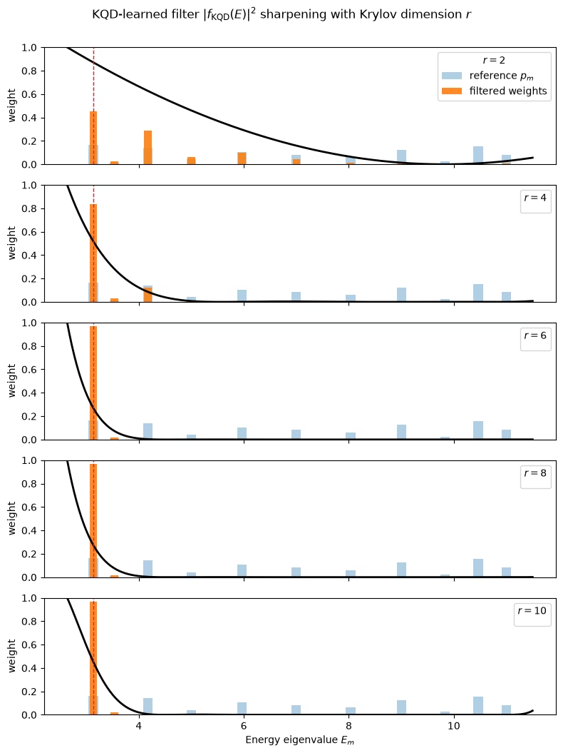
\begin{equation*} f_{\rm KQD}(E)=\sum_{\ell=0}^{r-1} c_\ell\, e^{-i\ell\Delta t E}, \end{equation*}

uma função trigonométrica da energia cujos coeficientes $\{c_\ell\}$ são precisamente o autovetor do GEVP resolvido acima. Minimizar o quociente de Rayleigh $\mathbf{c}^\dagger\mathcal{H}\mathbf{c}/\mathbf{c}^\dagger\mathcal{S}\mathbf{c}$ é, portanto, o mesmo que aprender o filtro que melhor suprime o peso do estado excitado da referência. Uma dimensão de Krylov $r$ maior dá ao filtro mais graus de liberdade e um pico mais nítido na energia do estado fundamental.

O auxiliar abaixo avalia este filtro aprendido em um eixo de energia; então o aplicamos à distribuição de referência obtida acima.

def trigonometric_krylov_filter(
    coeffs: np.ndarray,
    energies: np.ndarray,
    time_step: float,
) -> np.ndarray:
    """Evaluate the learned Krylov filter f(E) = sum_l c_l exp(-i l dt E)."""
    values = np.zeros_like(energies, dtype=complex)
    for ell, coeff in enumerate(coeffs):
        values += coeff * np.exp(-1j * ell * time_step * energies)
    return values

def filtered_spectral_weights(
    weights: np.ndarray,
    filter_values: np.ndarray,
) -> np.ndarray:
    """Reshape spectral weights by |f(E)|^2 and renormalize."""
    reshaped = weights * np.abs(filter_values) ** 2
    return reshaped / np.sum(reshaped)

# Recover the KQD coefficients from the already-estimated projected matrices.
# The shift only moves H by tau * S, so it does not change the GEVP eigenvector;
# we solve at the full Krylov dimension used in the small-scale example.
_, kqd_coeffs, _ = solve_thresholded_gevp(
    h_matrix_est,
    s_matrix_est,
    threshold=1e-12,
)

filter_on_spectrum = trigonometric_krylov_filter(
    kqd_coeffs, subspace_evals, dt
)
filtered_weights = filtered_spectral_weights(
    ref_spectral_weights, filter_on_spectrum
)

print(f"Ground-state overlap  (reference): {ref_spectral_weights[0]:.4f}")
print(f"Ground-state overlap  (filtered):  {filtered_weights[0]:.4f}")
print(
    f"Mean energy           (reference): {np.sum(ref_spectral_weights * subspace_evals):.6f}"
)
print(
    f"Mean energy           (filtered):  {np.sum(filtered_weights * subspace_evals):.6f}"
)

Ground-state overlap  (reference): 0.1638
Ground-state overlap  (filtered):  0.9638
Mean energy           (reference): 7.000000
Mean energy           (filtered):  3.164503

Visualize o filtro e sua flexibilidade

Primeiro mostramos o filtro aprendido na dimensão de Krylov completa usada acima, e então acompanhamos como ele se torna mais nítido à medida que a dimensão $r$ cresce.

As barras mostram os pesos espectrais de referência $p_m$ (antes) e os pesos filtrados $p_m|f_{\rm KQD}(E_m)|^2$ (depois), junto com a intensidade do filtro aprendido $|f_{\rm KQD}(E)|^2$ em um eixo de energia contínuo. O filtro concentra o peso na energia mais baixa do subespaço de excitação única — a mesma energia para a qual a estimativa KQD convergiu no exemplo em pequena escala. Observe que este é o estado fundamental dentro do setor de excitação única, que é o alvo relevante para este estado de referência que conserva excitações, não o estado fundamental global.

fig, ax = plt.subplots(figsize=(8, 4))

visible = (ref_spectral_weights > 1e-4) | (filtered_weights > 1e-4)
ax.bar(
    subspace_evals[visible],
    ref_spectral_weights[visible],
    width=0.18,
    alpha=0.45,
    label="reference $p_m$",
)
ax.bar(
    subspace_evals[visible],
    filtered_weights[visible],
    width=0.14,
    alpha=0.9,
    label=r"filtered $p_m\,|f_{\rm KQD}(E_m)|^2$",
)

energy_grid = np.linspace(
    subspace_evals.min() - 0.5, subspace_evals.max() + 0.5, 800
)
filter_intensity = (
    np.abs(trigonometric_krylov_filter(kqd_coeffs, energy_grid, dt)) ** 2
)
filter_intensity /= filter_intensity.max()
ax.plot(
    energy_grid,
    filter_intensity,
    color="k",
    linewidth=2,
    label=r"$|f_{\rm KQD}(E)|^2$ (normalized)",
)

ax.axvline(
    subspace_evals[0],
    color="C3",
    linestyle="--",
    linewidth=1,
    label="subspace ground energy",
)
ax.set_xlabel("Energy eigenvalue $E_m$")
ax.set_ylabel("Spectral weight")
ax.set_ylim(0, 1)
ax.legend(loc="upper right")
plt.tight_layout()
plt.show()

Output of the previous code cell

Aumentando a dimensão de Krylov: flexibilidade da função aprendida

Lembre-se de que o filtro aprendido é um polinômio trigonométrico na energia com $r$ coeficientes,

\begin{equation*} f_{\rm KQD}(E)=\sum_{\ell=0}^{r-1} c_\ell\, e^{-i\ell\Delta t E}. \end{equation*}

A dimensão de Krylov $r$ é exatamente o número de coeficientes livres, então ela controla a flexibilidade da função. Um $r$ pequeno só pode produzir um filtro amplo e suavemente variável que vaza peso para estados excitados de baixa energia; quando $r$ aumenta, o filtro pode formar um pico mais estreito na energia alvo e suprimir o peso restante do estado excitado de forma mais agressiva. Este é o análogo, do ponto de vista do filtro espectral, da convergência de energia observada no exemplo em pequena escala: à medida que $r$ cresce, a distribuição filtrada colapsa sobre o estado fundamental do subespaço e a energia estimada diminui em direção a ele.

Reutilizamos as matrizes projetadas já estimadas acima e simplesmente resolvemos o GEVP em cada bloco principal $r\times r$ , e então avaliamos e plotamos o filtro correspondente.

# Sweep the Krylov dimension using the leading r x r blocks of the estimated matrices.
sweep_dims = [r for r in (2, 4, 6, 8, krylov_dim) if r <= krylov_dim]
sweep_dims = sorted(set(sweep_dims))

energy_grid = np.linspace(
    subspace_evals.min() - 0.5, subspace_evals.max() + 0.5, 800
)

sweep_cases = []
print(" r    retained    ground overlap    filtered energy")
print("--    --------    --------------    ---------------")
for r in sweep_dims:
    _, coeffs_r, retained_r = solve_thresholded_gevp(
        h_matrix_est[:r, :r],
        s_matrix_est[:r, :r],
        threshold=1e-12,
    )
    filter_on_spectrum_r = trigonometric_krylov_filter(
        coeffs_r, subspace_evals, dt
    )
    filtered_weights_r = filtered_spectral_weights(
        ref_spectral_weights, filter_on_spectrum_r
    )
    filtered_energy_r = float(np.sum(filtered_weights_r * subspace_evals))

    sweep_cases.append((r, coeffs_r, filtered_weights_r))
    print(
        f"{r:2d}    {retained_r:8d}    {filtered_weights_r[0]:14.4f}    {filtered_energy_r:15.6f}"
    )

print(f"\nSubspace ground-state energy (target): {subspace_evals[0]:.6f}")

# One panel per Krylov dimension: filtered spectrum (bars) + filter intensity (curve).
fig, axes = plt.subplots(
    len(sweep_cases),
    1,
    figsize=(8, 2.1 * len(sweep_cases)),
    sharex=True,
)
axes = np.atleast_1d(axes)

for idx, (ax, (r, coeffs_r, filtered_weights_r)) in enumerate(
    zip(axes, sweep_cases)
):
    visible = (ref_spectral_weights > 1e-4) | (filtered_weights_r > 1e-4)
    ax.bar(
        subspace_evals[visible],
        ref_spectral_weights[visible],
        width=0.18,
        alpha=0.35,
        color="C0",
        label="reference $p_m$" if idx == 0 else None,
    )
    ax.bar(
        subspace_evals[visible],
        filtered_weights_r[visible],
        width=0.14,
        alpha=0.9,
        color="C1",
        label="filtered weights" if idx == 0 else None,
    )

    filter_intensity_r = (
        np.abs(trigonometric_krylov_filter(coeffs_r, energy_grid, dt)) ** 2
    )
    filter_intensity_r /= filter_intensity_r.max()
    ax.plot(energy_grid, filter_intensity_r, color="k", linewidth=2)

    ax.axvline(subspace_evals[0], color="C3", linestyle="--", linewidth=1)
    ax.set_ylim(0, 1)
    ax.set_ylabel("weight")
    ax.legend(loc="upper right", title=f"$r={r}$")

axes[-1].set_xlabel("Energy eigenvalue $E_m$")
fig.suptitle(
    r"KQD-learned filter $|f_{\rm KQD}(E)|^2$ sharpening with Krylov dimension $r$",
    y=1.0,
)
fig.tight_layout()
plt.show()

r    retained    ground overlap    filtered energy
--    --------    --------------    ---------------
 2           2            0.4549           4.184510
 4           4            0.8373           3.310168
 6           6            0.9706           3.158100
 8           7            0.9701           3.158725
10           8            0.9638           3.164503

Subspace ground-state energy (target): 3.136297

Output of the previous code cell

Próximos passos

Se você achou este trabalho interessante, pode se interessar pelo seguinte material:

Recomendações

Referências

[1] E. N. Epperly, L. Lin, and Y. Nakatsukasa, A theory of quantum subspace diagonalization, SIAM Journal on Matrix Analysis and Applications 43, 1263-1290 (2022).

[2] N. Yoshioka, M. Amico, W. Kirby, et al., Diagonalization of large many-body Hamiltonians on a quantum processor, arXiv:2407.14431 (2024).

[3] R. M. Parrish e P. L. McMahon, Quantum filter diagonalization: quantum eigendecomposition without full quantum phase estimation, Physical Review Letters 122, 230401 (2019).

[4] G. Lee, S. Choi, J. Huh, e A. F. Izmaylov, Efficient strategies for reducing sampling error in quantum Krylov subspace diagonalization, Digital Discovery 4, 954-969 (2025).

[5] G. Lee, M. Kang, J. Hong, S. Fomichev e J. Huh, Filtered Quantum Phase Estimation, arXiv:2510.04294 (2025).

Resultados de aprendizagem​

Pré-requisitos​

Contexto​

Requisitos​

Configuração​

Exemplo de simulador em pequena escala​

Etapa 1: Mapear entradas clássicas para um problema quântico​

Hamiltoniano e estado de referência​

Definir os parâmetros do algoritmo​

Construir circuito​

Estado de referência​

Evolução temporal​

Circuito de teste de troca estendido [3]​

Observáveis​

Etapa 2: Otimizar o problema para execução em hardware quântico​

Comparar a ordenação de termos Hamiltonianos​

Comparar a síntese de fórmula de produto​

Remover a porta de evolução temporal controlada​

Transpilação​

Etapa 3: Executar usando primitivas do Qiskit​

Etapa 4: Pós-processar e retornar o resultado no formato clássico desejado​

Exemplo de hardware em larga escala​

Passos 1-4 comprimidos em um único bloco de código​

Apêndice: A perspectiva da função hamiltoniana (filtro espectral)​

O estado de referência como uma distribuição de energia​

O KQD aprende um filtro que remodela esta distribuição​

Visualize o filtro e sua flexibilidade​

Aumentando a dimensão de Krylov: flexibilidade da função aprendida​

Próximos passos​

Referências​

Resultados de aprendizagem

Pré-requisitos

Contexto

Requisitos

Configuração

Exemplo de simulador em pequena escala

Etapa 1: Mapear entradas clássicas para um problema quântico

Hamiltoniano e estado de referência

Definir os parâmetros do algoritmo

Construir circuito

Estado de referência

Evolução temporal

Circuito de teste de troca estendido [3]

Observáveis

Etapa 2: Otimizar o problema para execução em hardware quântico

Comparar a ordenação de termos Hamiltonianos

Comparar a síntese de fórmula de produto

Remover a porta de evolução temporal controlada

Transpilação

Etapa 3: Executar usando primitivas do Qiskit

Etapa 4: Pós-processar e retornar o resultado no formato clássico desejado

Exemplo de hardware em larga escala

Passos 1-4 comprimidos em um único bloco de código

Apêndice: A perspectiva da função hamiltoniana (filtro espectral)

O estado de referência como uma distribuição de energia

O KQD aprende um filtro que remodela esta distribuição

Visualize o filtro e sua flexibilidade

Aumentando a dimensão de Krylov: flexibilidade da função aprendida

Próximos passos

Referências