Experimento em escala de utilidade III

nota

Toshinari Itoko, Tamiya Onodera, Kifumi Numata (19 de julho de 2024)

Baixe o PDF da aula original. Alguns trechos de código podem estar desatualizados, pois são imagens estáticas.

O tempo aproximado de QPU para executar este primeiro experimento é de 12 min 30 s. Há um experimento adicional abaixo que requer aproximadamente 4 min.

(Observação: este notebook pode não ser executado dentro do tempo permitido no Plano Open. Use os recursos de computação quântica com sabedoria.)

# Added by doQumentation — required packages for this notebook
!pip install -q numpy qiskit qiskit-ibm-runtime rustworkx

import qiskit

qiskit.__version__

'2.0.2'

import qiskit_ibm_runtime

qiskit_ibm_runtime.__version__

'0.40.1'

import numpy as np
import rustworkx as rx

from qiskit import QuantumCircuit
from qiskit.visualization import plot_histogram
from qiskit.visualization import plot_gate_map
from qiskit.transpiler.preset_passmanagers import generate_preset_pass_manager
from qiskit.providers import BackendV2
from qiskit.quantum_info import SparsePauliOp

from qiskit_ibm_runtime import QiskitRuntimeService
from qiskit_ibm_runtime import Sampler, Estimator, Batch, SamplerOptions

1. Introdução

Vamos fazer uma breve revisão dos estados GHZ e do tipo de distribuição que você pode esperar ao aplicar o Sampler a um deles. Em seguida, definiremos explicitamente o objetivo desta lição.

1.1 Estado GHZ

O estado GHZ (estado de Greenberger-Horne-Zeilinger) para $n$ qubits é definido como

$$\frac{1}{\sqrt 2}(|0\rangle ^ {\otimes n}+ |1\rangle^ {\otimes n})$$

Naturalmente, ele pode ser criado para 6 qubits com o seguinte circuito quântico.

N = 6
qc = QuantumCircuit(N, N)

qc.h(0)
for i in range(N - 1):
    qc.cx(0, i + 1)

# qc.measure_all()
qc.barrier()
qc.measure(list(range(N)), list(range(N)))

qc.draw(output="mpl", idle_wires=False, scale=0.5)

print("Depth:", qc.depth())

Depth: 7

A profundidade não é muito grande, embora você saiba, pelas lições anteriores, que dá para fazer melhor. Vamos escolher um backend e transpilar este circuito.

service = QiskitRuntimeService()
backend = service.least_busy(operational=True, simulator=False)
backend.name
# or
# backend = service.least_busy(operational=True)
# backend.name

'ibm_kingston'

pm = generate_preset_pass_manager(3, backend=backend)
qc_transpiled = pm.run(qc)
qc_transpiled.draw(output="mpl", idle_wires=False, fold=-1)

print("Depth:", qc_transpiled.depth())
print(
    "Two-qubit Depth:",
    qc_transpiled.depth(filter_function=lambda x: x.operation.num_qubits == 2),
)

Depth: 27
Two-qubit Depth: 11

Novamente, a profundidade de dois qubits após a transpilação não é muito grande. Mas para trabalhar com um estado GHZ em mais qubits, você precisará claramente pensar em otimizar o circuito. Vamos executar isso usando o Sampler e ver o que um computador quântico real retorna.

sampler = Sampler(mode=backend)
shots = 40000
job = sampler.run([qc_transpiled], shots=shots)
job_id = job.job_id()
print(job_id)

d147y20n2txg008jvv70

job.status()

'DONE'

job = service.job(job_id)
result = job.result()
plot_histogram(result[0].data.c.get_counts(), figsize=(30, 5))

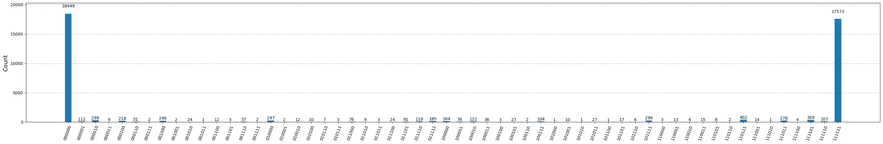
Este é o resultado do circuito GHZ de 6 qubits. Como você pode ver, os estados de todos os $|0\rangle$'s e todos os $|1\rangle$'s dominam, mas os erros são substanciais. Vamos tentar ver qual é o maior circuito GHZ que você consegue construir com um dispositivo Eagle, mantendo os estados corretos com probabilidade de pelo menos 50%.

1.2 Seu objetivo

Construa um circuito GHZ para 20 qubits ou mais de modo que, ao medir, a fidelidade do seu estado GHZ seja > 0,5. Observações:

• Você precisa usar um dispositivo Eagle (min_num_qubits=127) e definir o número de shots como 40.000.
• Você deve executar o circuito GHZ usando a função execute_ghz_fidelity e calcular a fidelidade usando a função check_ghz_fidelity_from_jobs.

Este é um exercício independente, no qual você aproveita o que aprendeu até agora neste curso.

def execute_ghz_fidelity(
    ghz_circuit: QuantumCircuit,  # Quantum circuit to create GHZ state (Circuit after Routing or without Routing), Classical register name is "c"
    physical_qubits: list[int],  # Physical qubits to represent GHZ state
    backend: BackendV2,
    sampler_options: dict | SamplerOptions | None = None,
):
    N_SHOTS = 40_000
    N = len(physical_qubits)
    base_circuit = ghz_circuit.remove_final_measurements(inplace=False)
    # M_k measurement circuits
    mk_circuits = []
    for k in range(1, N + 1):
        circuit = base_circuit.copy()
        # change measurement basis
        for q in physical_qubits:
            circuit.rz(-k * np.pi / N, q)
            circuit.h(q)
        mk_circuits.append(circuit)

    obs = SparsePauliOp.from_sparse_list(
        [("Z" * N, physical_qubits, 1)], num_qubits=backend.num_qubits
    )
    job_ids = []
    pm1 = generate_preset_pass_manager(1, backend=backend)
    org_transpiled = pm1.run(ghz_circuit)
    mk_transpiled = pm1.run(mk_circuits)
    with Batch(backend=backend):
        sampler = Sampler(options=sampler_options)
        sampler.options.twirling.enable_measure = True
        job = sampler.run([org_transpiled], shots=N_SHOTS)
        job_ids.append(job.job_id())
        # print(f"Sampler job id: {job.job_id()}, shots={N_SHOTS}")
        estimator = Estimator()  # TREX is applied as default
        estimator.options.dynamical_decoupling.enable = True
        estimator.options.execution.rep_delay = 0.0005
        estimator.options.twirling.enable_measure = True
        job2 = estimator.run([(circ, obs) for circ in mk_transpiled], precision=1 / 100)
        job_ids.append(job2.job_id())
        # print("Estimator job id:", job2.job_id())
        return [job.job_id(), job2.job_id()]

def check_ghz_fidelity_from_jobs(
    sampler_job,
    estimator_job,
    num_qubits,
    shots=40_000,
):
    N = num_qubits
    sampler_result = sampler_job.result()
    counts = sampler_result[0].data.c.get_counts()
    all_zero = counts.get("0" * N, 0) / shots
    all_one = counts.get("1" * N, 0) / shots
    top3 = sorted(counts, key=counts.get, reverse=True)[:3]
    print(
        f"N={N}: |00..0>: {counts.get('0'*N, 0)}, |11..1>: {counts.get('1'*N, 0)}, |3rd>: {counts.get(top3[2], 0)} ({top3[2]})"
    )
    print(f"P(|00..0>)={all_zero}, P(|11..1>)={all_one}")

    estimator_result = estimator_job.result()
    non_diagonal = (1 / N) * sum(
        (-1) ** k * estimator_result[k - 1].data.evs for k in range(1, N + 1)
    )
    print(f"REM: Coherence (non-diagonal): {non_diagonal:.6f}")
    fidelity = 0.5 * (all_zero + all_one + non_diagonal)
    sigma = 0.5 * np.sqrt(
        (1 - all_zero - all_one) * (all_zero + all_one) / shots
        + sum(estimator_result[k].data.stds ** 2 for k in range(N)) / (N * N)
    )
    print(f"GHZ fidelity = {fidelity:.6f} ± {sigma:.6f}")
    if fidelity - 2 * sigma > 0.5:
        print("GME (genuinely multipartite entangled) test: Passed")
    else:
        print("GME (genuinely multipartite entangled) test: Failed")
    return {
        "fidelity": fidelity,
        "sigma": sigma,
        "shots": shots,
        "job_ids": [sampler_job.job_id(), estimator_job.job_id()],
    }

Neste notebook, aplicaremos três estratégias para criar bons estados GHZ usando 16 qubits e 30 qubits. Essas abordagens se baseiam em estratégias que você já conhece das lições anteriores.

2. Estratégia 1: Seleção de qubits com consciência de ruído

Primeiro, especificamos um backend. Como vamos trabalhar extensivamente com as propriedades de um backend específico, faz sentido definir um backend fixo, em vez de usar a opção least_busy.

backend = service.backend("ibm_strasbourg")  # eagle
twoq_gate = "ecr"
print(f"Device {backend.name} Loaded with {backend.num_qubits} qubits")
print(f"Two Qubit Gate: {twoq_gate}")

Device ibm_strasbourg Loaded with 127 qubits
Two Qubit Gate: ecr

Vamos construir um circuito com muitas portas de dois qubits. Faz sentido usar os qubits que apresentam os menores erros ao implementar essas portas de dois qubits. Encontrar a melhor "cadeia de qubits" com base nos erros de porta 2q reportados é um problema não trivial. Mas podemos definir algumas funções para nos ajudar a determinar os melhores qubits a usar.

coupling_map = backend.target.build_coupling_map(twoq_gate)
G = coupling_map.graph

def to_edges(path):  # create edges list from node paths
    edges = []
    prev_node = None
    for node in path:
        if prev_node is not None:
            if G.has_edge(prev_node, node):
                edges.append((prev_node, node))
            else:
                edges.append((node, prev_node))
        prev_node = node
    return edges

def path_fidelity(path, correct_by_duration: bool = True, readout_scale: float = None):
    """Compute an estimate of the total fidelity of 2-qubit gates on a path.
    If `correct_by_duration` is true, each gate fidelity is worsen by
    scale = max_duration / duration, that is, gate_fidelity^scale.
    If `readout_scale` > 0 is supplied, readout_fidelity^readout_scale
    for each qubit on the path is multiplied to the total fielity.
    The path is given in node indices form, for example, [0, 1, 2].
    An external function `to_edges` is used to obtain edge list, for example, [(0, 1), (1, 2)]."""
    path_edges = to_edges(path)
    max_duration = max(backend.target[twoq_gate][qs].duration for qs in path_edges)

    def gate_fidelity(qpair):
        duration = backend.target[twoq_gate][qpair].duration
        scale = max_duration / duration if correct_by_duration else 1.0
        # 1.25 = (d+1)/d with d = 4
        return max(0.25, 1 - (1.25 * backend.target[twoq_gate][qpair].error)) ** scale

    def readout_fidelity(qubit):
        return max(0.25, 1 - backend.target["measure"][(qubit,)].error)

    total_fidelity = np.prod(
        [gate_fidelity(qs) for qs in path_edges]
    )  # two qubits gate fidelity for each path
    if readout_scale:
        total_fidelity *= (
            np.prod([readout_fidelity(q) for q in path]) ** readout_scale
        )  # multiply readout fidelity
    return total_fidelity

def flatten(paths, cutoff=None):  # cutoff is for not making run time too large
    return [
        path
        for s, s_paths in paths.items()
        for t, st_paths in s_paths.items()
        for path in st_paths[:cutoff]
        if s < t
    ]

N = 16  # Number of qubits to use in the GHZ circuit
num_qubits_in_chain = N

Vamos usar as funções acima para encontrar todos os caminhos simples de N qubits entre todos os pares de nós no grafo (Referência: all_pairs_all_simple_paths).

Em seguida, usando a função path_fidelity criada acima, encontraremos a melhor cadeia de qubits que possui a maior fidelidade de caminho.

from functools import partial

%%time
paths = rx.all_pairs_all_simple_paths(
    G.to_undirected(multigraph=False),
    min_depth=num_qubits_in_chain,
    cutoff=num_qubits_in_chain,
)
paths = flatten(paths, cutoff=25)  # If you have time, you could set a larger cutoff.
if not paths:
    raise Exception(
        f"No qubit chain with length={num_qubits_in_chain} exists in {backend.name}. Try smaller num_qubits_in_chain."
    )

print(f"Selecting the best from {len(paths)} candidate paths")

best_qubit_chain = max(
    paths, key=partial(path_fidelity, correct_by_duration=True, readout_scale=1.0)
)
assert len(best_qubit_chain) == num_qubits_in_chain
print(f"Predicted (best possible) process fidelity: {path_fidelity(best_qubit_chain)}")

Selecting the best from 6046 candidate paths
Predicted (best possible) process fidelity: 0.8929026784775056
CPU times: user 284 ms, sys: 10.9 ms, total: 295 ms
Wall time: 295 ms

np.array(best_qubit_chain)

array([55, 49, 48, 47, 46, 45, 54, 64, 65, 66, 73, 85, 86, 87, 88, 89],
      dtype=uint64)

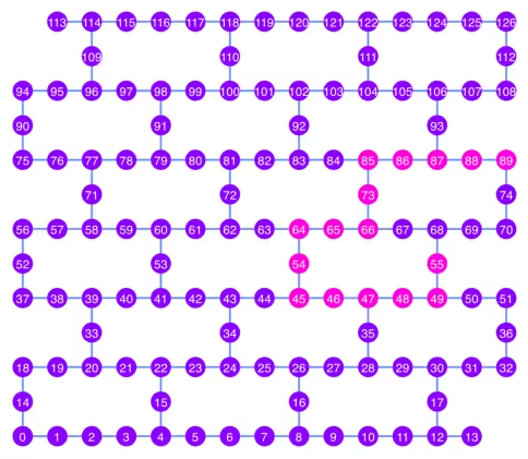
Vamos plotar a melhor cadeia de qubits, mostrada em rosa, no diagrama do mapa de acoplamento.

qubit_color = []
for i in range(133):
    if i in best_qubit_chain:
        qubit_color.append("#ff00dd")  # pink
    else:
        qubit_color.append("#8c00ff")  # purple
plot_gate_map(
    backend, qubit_color=qubit_color, qubit_size=50, font_size=25, figsize=(6, 6)
)

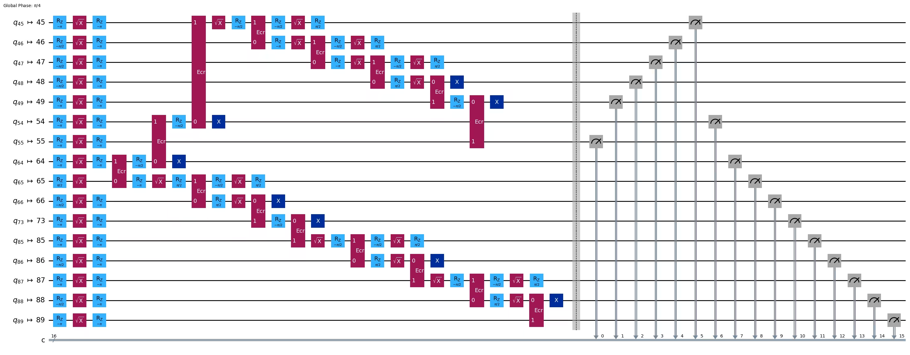
2.1 Construindo um circuito GHZ na melhor cadeia de qubits

Escolhemos um qubit no meio da cadeia para aplicar primeiro a porta H. Isso deve reduzir a profundidade do circuito em aproximadamente metade.

ghz1 = QuantumCircuit(max(best_qubit_chain) + 1, N)
ghz1.h(best_qubit_chain[N // 2])
for i in range(N // 2, 0, -1):
    ghz1.cx(best_qubit_chain[i], best_qubit_chain[i - 1])
for i in range(N // 2, N - 1, +1):
    ghz1.cx(best_qubit_chain[i], best_qubit_chain[i + 1])
ghz1.barrier()  # for visualization
ghz1.measure(best_qubit_chain, list(range(N)))
ghz1.draw(output="mpl", idle_wires=False, scale=0.5, fold=-1)

ghz1.depth()

10

pm = generate_preset_pass_manager(1, backend=backend)
ghz1_transpiled = pm.run(ghz1)
ghz1_transpiled.draw(output="mpl", idle_wires=False, fold=-1)

print("Depth:", ghz1_transpiled.depth())
print(
    "Two-qubit Depth:",
    ghz1_transpiled.depth(filter_function=lambda x: x.operation.num_qubits == 2),
)

Depth: 27
Two-qubit Depth: 8

opts = SamplerOptions()

res = execute_ghz_fidelity(
    ghz_circuit=ghz1,
    physical_qubits=best_qubit_chain,
    backend=backend,
    sampler_options=opts,
)

job_s = service.job(res[0])  # Use your job id showed above.
job_e = service.job(res[1])
print(job_s.status(), job_e.status())

DONE DONE

Tenha cuidado para executar a próxima célula somente depois que os status dos jobs acima tiverem se tornado 'DONE', para exibir o resultado usando a função check_ghz_fidelity_from_jobs.

N = 16
# Check fidelity from job IDs
res = check_ghz_fidelity_from_jobs(
    sampler_job=job_s,
    estimator_job=job_e,
    num_qubits=N,
)

N=16: |00..0>: 153, |11..1>: 8681, |3rd>: 2262 (1111111111101111)
P(|00..0>)=0.003825, P(|11..1>)=0.217025
REM: Coherence (non-diagonal): 0.073809
GHZ fidelity = 0.147329 ± 0.002438
GME (genuinely multipartite entangled) test: Failed

result = job_s.result()
plot_histogram(result[0].data.c.get_counts(), figsize=(30, 5))

Este resultado não atende aos critérios. Vamos passar para a próxima ideia.

3. Estratégia 2: Árvore balanceada de qubits

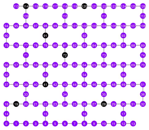
A próxima ideia é encontrar uma árvore balanceada de qubits. Usando a árvore em vez da cadeia, a profundidade do circuito deve ficar menor. Antes disso, removemos os nós com erros de leitura "ruins" e as arestas com erros de gate "ruins" do grafo de acoplamento.

BAD_READOUT_ERROR_THRESHOLD = 0.1
BAD_ECRGATE_ERROR_THRESHOLD = 0.1
bad_readout_qubits = [
    q
    for q in range(backend.num_qubits)
    if backend.target["measure"][(q,)].error > BAD_READOUT_ERROR_THRESHOLD
]
bad_ecrgate_edges = [
    qpair
    for qpair in backend.target["ecr"]
    if backend.target["ecr"][qpair].error > BAD_ECRGATE_ERROR_THRESHOLD
]
print("Bad readout qubits:", bad_readout_qubits)
print("Bad ECR gates:", bad_ecrgate_edges)

Bad readout qubits: [19, 28, 41, 72, 91, 114, 120]
Bad ECR gates: []

g = backend.coupling_map.graph.copy().to_undirected()
g.remove_edges_from(
    bad_ecrgate_edges
)  # remove edge first (otherwise might fail with a NoEdgeBetweenNodes error)
g.remove_nodes_from(bad_readout_qubits)

Vamos desenhar o grafo do mapa de acoplamento sem as arestas e os qubits ruins.

qubit_color = []
for i in range(133):
    if i in bad_readout_qubits:
        qubit_color.append("#000000")  # black
    else:
        qubit_color.append("#8c00ff")  # purple
line_color = []
for e in backend.target.build_coupling_map().get_edges():
    if e in bad_ecrgate_edges:
        line_color.append("#ffffff")  # white
    else:
        line_color.append("#888888")  # gray
plot_gate_map(
    backend,
    qubit_color=qubit_color,
    line_color=line_color,
    qubit_size=50,
    font_size=25,
    figsize=(6, 6),
)

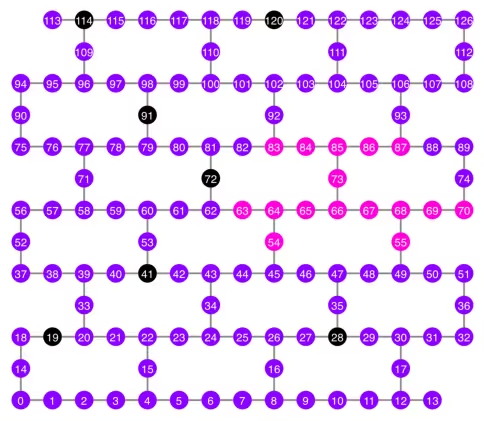
Vamos tentar criar um estado GHZ de 16 qubits como antes.

N = 16

Chamamos a função betweenness_centrality para encontrar um qubit para o nó raiz. O nó com o maior valor de centralidade de intermediação está no centro do grafo. Referência: https://www.rustworkx.org/tutorial/betweenness_centrality.html

Ou você pode selecioná-lo manualmente.

# central = 65 #Select the center node manually
c_degree = dict(rx.betweenness_centrality(g))
central = max(c_degree, key=c_degree.get)
central

66

Partindo do nó raiz, geramos uma árvore por busca em largura (BFS). Referência: https://qiskit.org/ecosystem/rustworkx/apiref/rustworkx.bfs_search.html#rustworkx-bfs-search

class TreeEdgesRecorder(rx.visit.BFSVisitor):
    def __init__(self, N):
        self.edges = []
        self.N = N

    def tree_edge(self, edge):
        self.edges.append(edge)
        if len(self.edges) >= self.N - 1:
            raise rx.visit.StopSearch()

vis = TreeEdgesRecorder(N)
rx.bfs_search(g, [central], vis)
best_qubits = sorted(list(set(q for e in vis.edges for q in (e[0], e[1]))))
# print('Tree edges:', vis.edges)

print("Qubits selected:", best_qubits)

Qubits selected: [54, 55, 63, 64, 65, 66, 67, 68, 69, 70, 73, 83, 84, 85, 86, 87]

Vamos plotar os qubits selecionados, mostrados em rosa, no diagrama do mapa de acoplamento.

qubit_color = []
for i in range(133):
    if i in bad_readout_qubits:
        qubit_color.append("#000000")  # black
    elif i in best_qubits:
        qubit_color.append("#ff00dd")  # pink
    else:
        qubit_color.append("#8c00ff")  # purple
plot_gate_map(
    backend,
    qubit_color=qubit_color,
    line_color=line_color,
    qubit_size=50,
    font_size=25,
    figsize=(6, 6),
)

Vamos mostrar a estrutura de árvore dos qubits.

from rustworkx.visualization import graphviz_draw

tree = rx.PyDiGraph()
tree.extend_from_weighted_edge_list(vis.edges)
tree.remove_nodes_from([n for n in range(max(best_qubits) + 1) if n not in best_qubits])

graphviz_draw(tree, method="dot")

ghz2 = QuantumCircuit(max(best_qubits) + 1, N)

ghz2.h(tree.edge_list()[0][0])  # apply H-gate to the root node
# Apply CNOT from the root node to the each edge.
for u, v in tree.edge_list():
    ghz2.cx(u, v)
ghz2.barrier()  # for visualization
ghz2.measure(best_qubits, list(range(N)))
ghz2.draw(output="mpl", idle_wires=False, scale=0.5)

ghz2.depth()

8

pm = generate_preset_pass_manager(1, backend=backend)
ghz2_transpiled = pm.run(ghz2)
ghz2_transpiled.draw(output="mpl", idle_wires=False, fold=-1)

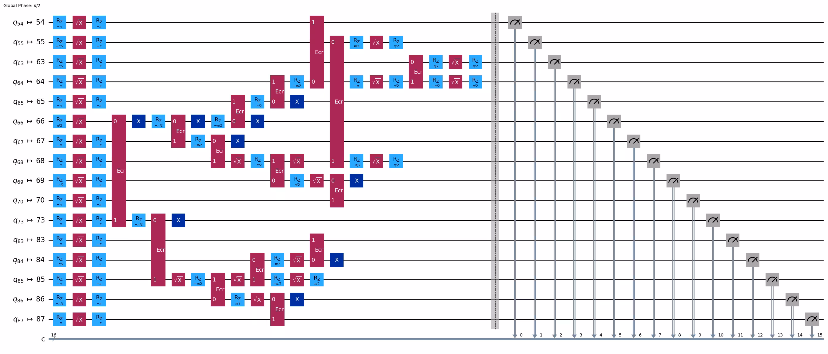
print("Depth:", ghz2_transpiled.depth())
print(
    "Two-qubit Depth:",
    ghz2_transpiled.depth(filter_function=lambda x: x.operation.num_qubits == 2),
)

Depth: 22
Two-qubit Depth: 6

A profundidade do circuito agora ficou muito menor do que a da estrutura em cadeia.

res = execute_ghz_fidelity(
    ghz_circuit=ghz2,
    physical_qubits=best_qubits,
    backend=backend,
    sampler_options=opts,
)

job_s = service.job(res[0])  # Use your job id showed above.
job_e = service.job(res[1])
print(job_s.status(), job_e.status())

DONE DONE

N = 16
# Check fidelity from job IDs
res = check_ghz_fidelity_from_jobs(
    sampler_job=job_s,
    estimator_job=job_e,
    num_qubits=N,
)

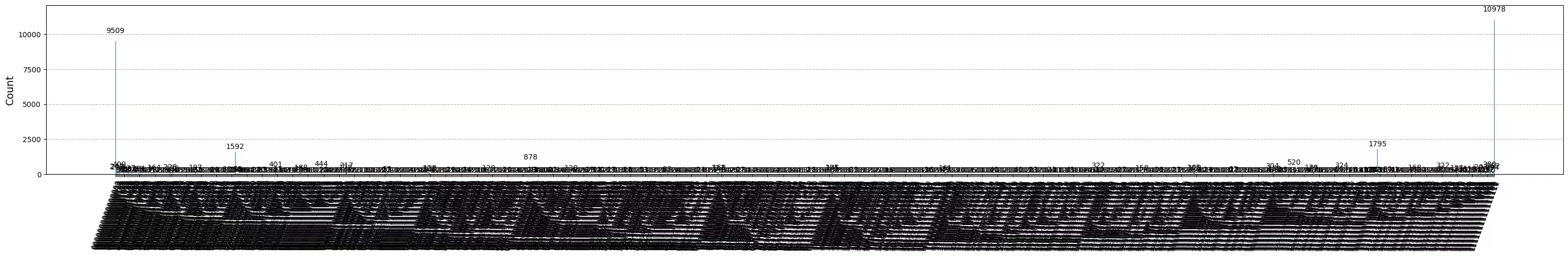
N=16: |00..0>: 9509, |11..1>: 10978, |3rd>: 1795 (1111110111111111)
P(|00..0>)=0.237725, P(|11..1>)=0.27445
REM: Coherence (non-diagonal): 0.606515
GHZ fidelity = 0.559345 ± 0.003188
GME (genuinely multipartite entangled) test: Passed

Passamos com sucesso nos critérios com a estrutura de árvore balanceada!

result = job_s.result()
plot_histogram(result[0].data.c.get_counts(), figsize=(30, 5))

Agora vamos tentar criar um estado GHZ maior: um estado GHZ de 30 qubits.

3.1 N = 30

Vamos seguir o framework Qiskit patterns.

• Passo 1: Mapear o problema para circuitos e operadores quânticos
• Passo 2: Otimizar para o hardware alvo
• Passo 3: Executar no hardware alvo
• Passo 4: Pós-processar os resultados

Passo 1: Mapear o problema para circuitos e operadores quânticos e Passo 2: Otimizar para o hardware alvo

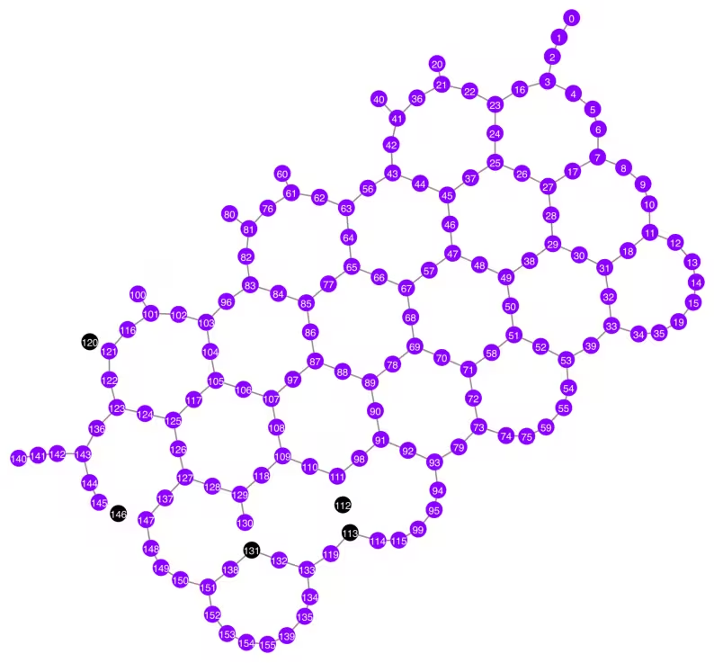
Aqui selecionamos o nó raiz manualmente.

central = 62  # Select the center node manually
# c_degree = dict(rx.betweenness_centrality(g))
# central = max(c_degree, key=c_degree.get)
# central

N = 30

vis = TreeEdgesRecorder(N)
rx.bfs_search(g, [central], vis)
best_qubits = sorted(list(set(q for e in vis.edges for q in (e[0], e[1]))))
print("Qubits selected:", best_qubits)

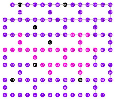
Qubits selected: [34, 35, 42, 43, 44, 45, 46, 47, 48, 53, 54, 56, 57, 58, 59, 60, 61, 62, 63, 64, 65, 66, 67, 68, 71, 73, 77, 84, 85, 86]

qubit_color = []
for i in range(133):
    if i in bad_readout_qubits:
        qubit_color.append("#000000")
    elif i in best_qubits:
        qubit_color.append("#ff00dd")
    else:
        qubit_color.append("#8c00ff")
line_color = []
for e in backend.target.build_coupling_map().get_edges():
    if e in bad_ecrgate_edges:
        line_color.append("#ffffff")
    else:
        line_color.append("#888888")
plot_gate_map(
    backend,
    qubit_color=qubit_color,
    line_color=line_color,
    qubit_size=50,
    font_size=25,
    figsize=(6, 6),
)

from rustworkx.visualization import graphviz_draw

tree = rx.PyDiGraph()
tree.extend_from_weighted_edge_list(vis.edges)
tree.remove_nodes_from([n for n in range(max(best_qubits) + 1) if n not in best_qubits])

graphviz_draw(tree, method="dot")

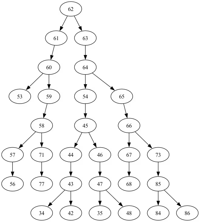
A profundidade desta árvore é 5.

ghz3 = QuantumCircuit(max(best_qubits) + 1, N)

ghz3.h(tree.edge_list()[0][0])  # apply H-gate to the root node
# Apply CNOT from the root node to the each edge.
for u, v in tree.edge_list():
    ghz3.cx(u, v)
ghz3.barrier()  # for visualization
ghz3.measure(best_qubits, list(range(N)))
ghz3.draw(output="mpl", idle_wires=False, fold=-1)

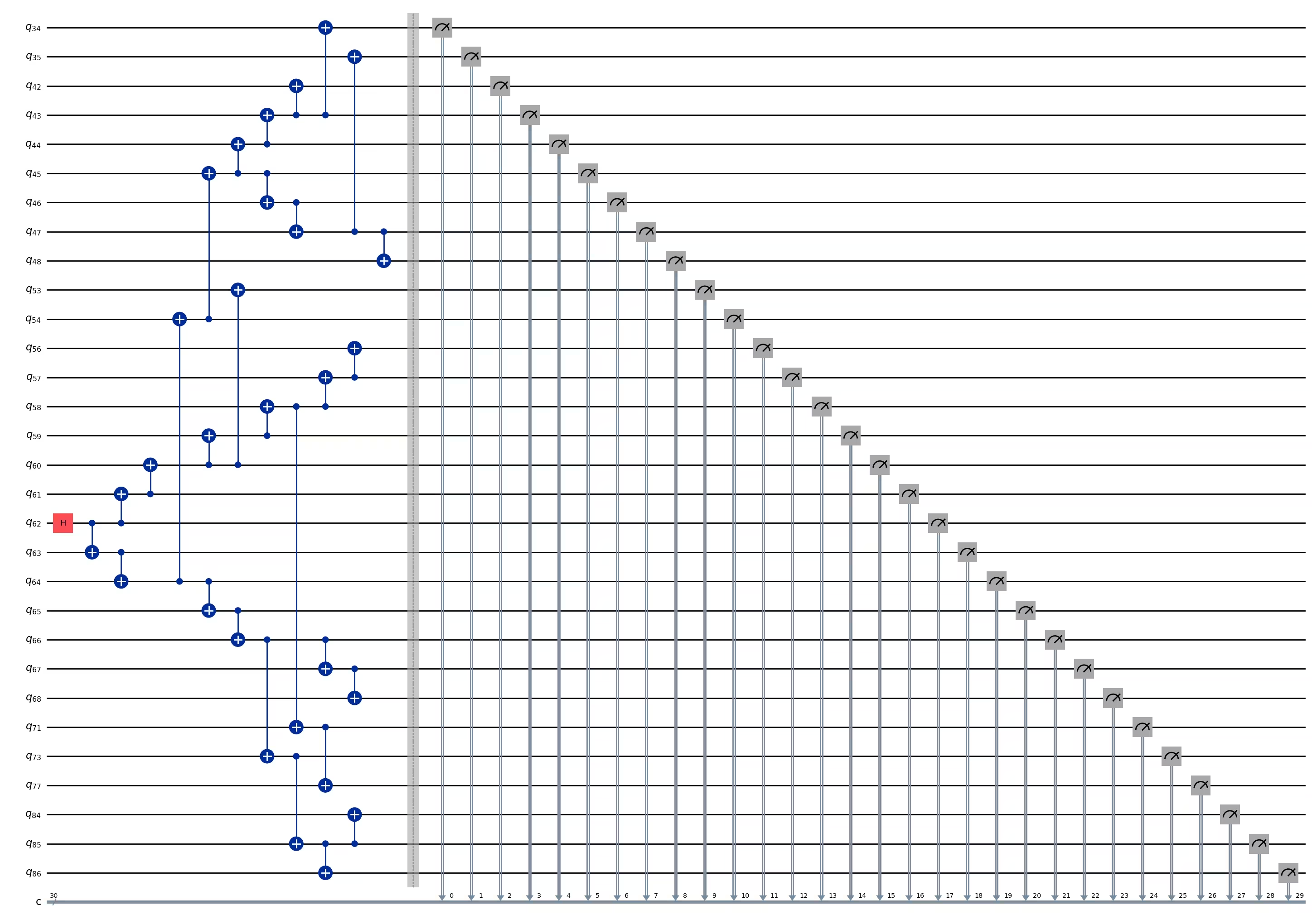
ghz3.depth()

11

pm = generate_preset_pass_manager(1, backend=backend)
ghz3_transpiled = pm.run(ghz3)
ghz3_transpiled.draw(output="mpl", idle_wires=False, fold=-1)

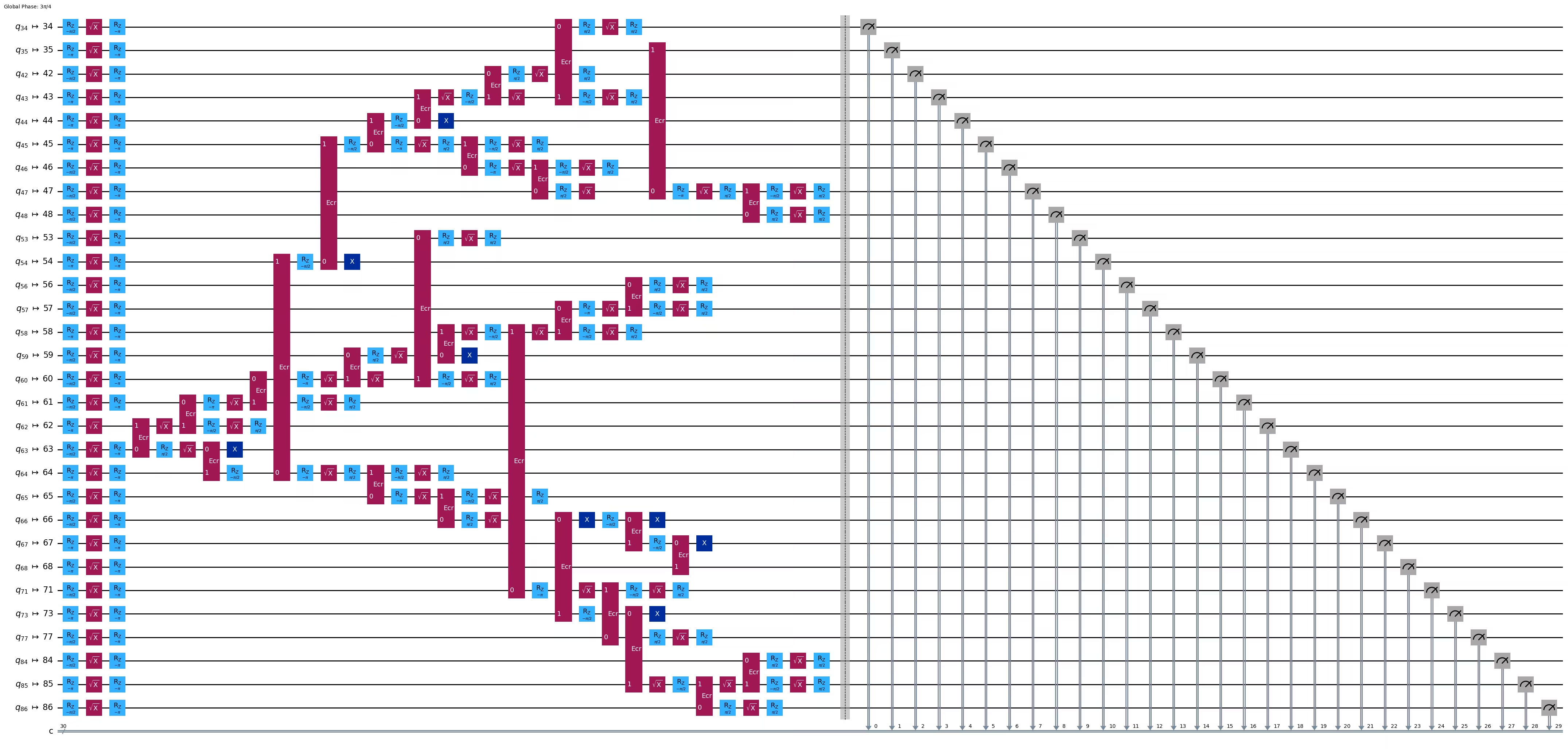
print("Depth:", ghz3_transpiled.depth())
print(
    "Two-qubit Depth:",
    ghz3_transpiled.depth(filter_function=lambda x: x.operation.num_qubits == 2),
)

Depth: 31
Two-qubit Depth: 9

3.2 Selecionar um nó raiz diferente manualmente

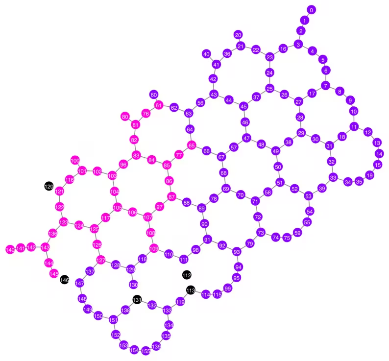
central = 54

vis = TreeEdgesRecorder(N)
rx.bfs_search(g, [central], vis)
best_qubits = sorted(list(set(q for e in vis.edges for q in (e[0], e[1]))))
print("Qubits selected:", best_qubits)

Qubits selected: [23, 24, 25, 34, 35, 42, 43, 44, 45, 46, 47, 48, 49, 50, 54, 55, 60, 61, 62, 63, 64, 65, 66, 67, 68, 69, 73, 84, 85, 86]

from rustworkx.visualization import graphviz_draw

tree = rx.PyDiGraph()
tree.extend_from_weighted_edge_list(vis.edges)
tree.remove_nodes_from([n for n in range(max(best_qubits) + 1) if n not in best_qubits])

graphviz_draw(tree, method="dot")

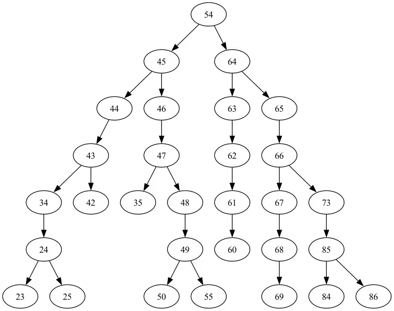
A profundidade desta árvore é 6.

ghz3 = QuantumCircuit(max(best_qubits) + 1, N)

ghz3.h(tree.edge_list()[0][0])  # apply H-gate to the root node
# Apply CNOT from the root node to the each edge.
for u, v in tree.edge_list():
    ghz3.cx(u, v)
ghz3.barrier()  # for visualization
ghz3.measure(best_qubits, list(range(N)))
ghz3.draw(output="mpl", idle_wires=False, fold=-1)

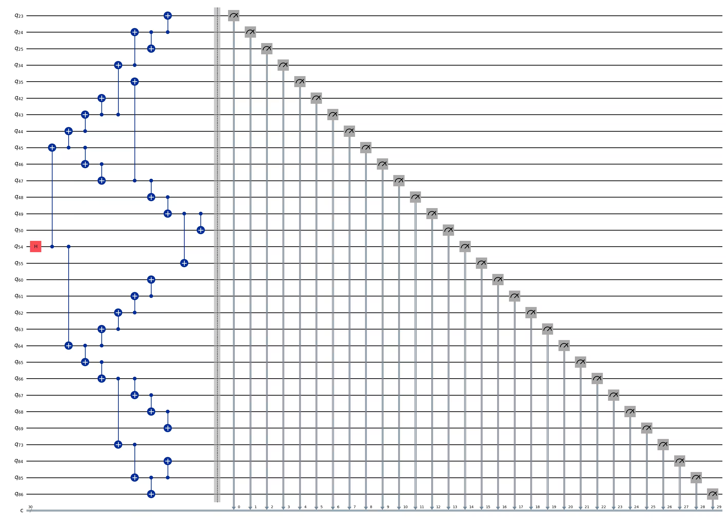
ghz3.depth()

11

pm = generate_preset_pass_manager(1, backend=backend)
ghz3_transpiled = pm.run(ghz3)
ghz3_transpiled.draw(output="mpl", idle_wires=False, fold=-1)

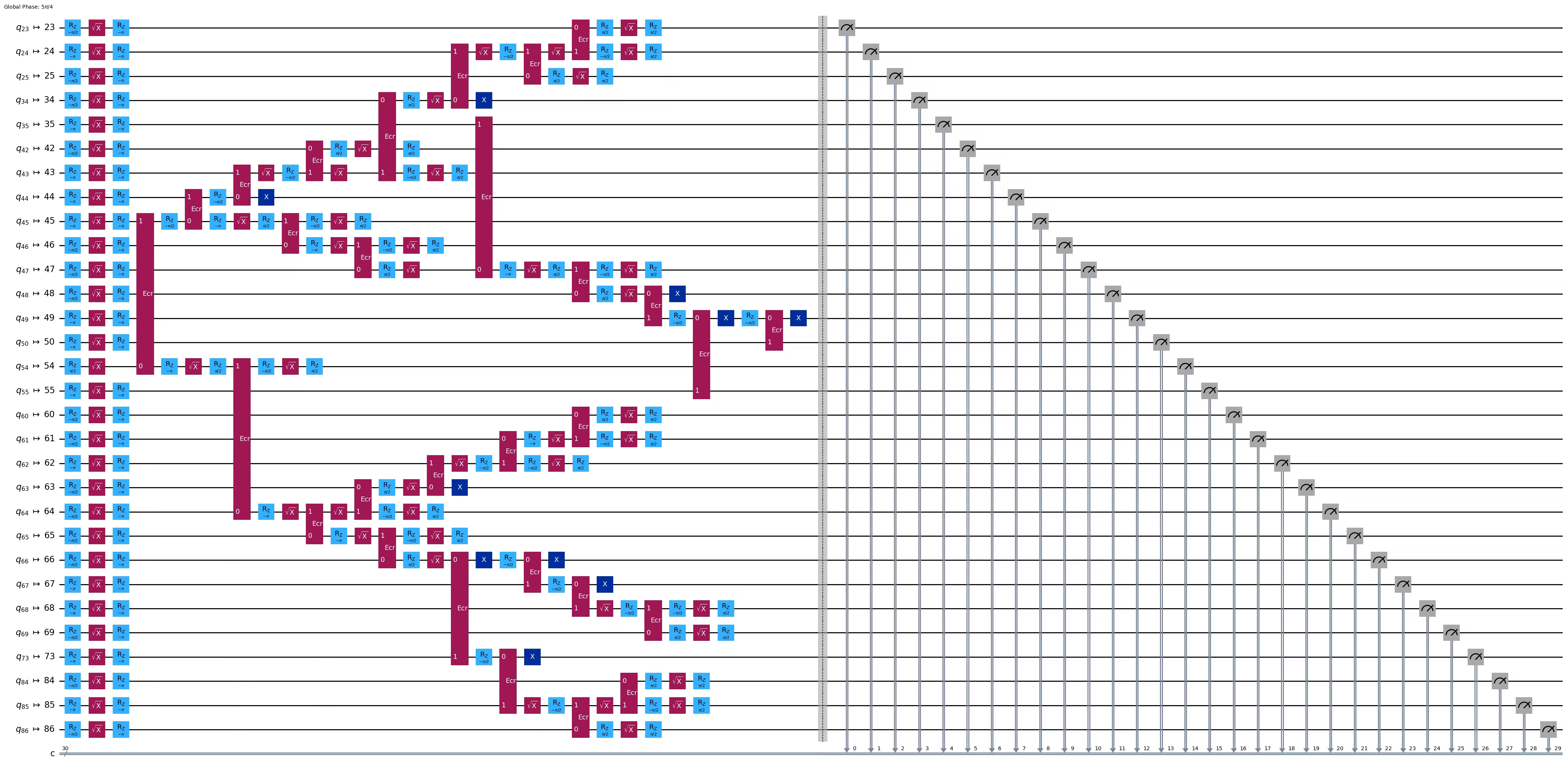
print("Depth:", ghz3_transpiled.depth())
print(
    "Two-qubit Depth:",
    ghz3_transpiled.depth(filter_function=lambda x: x.operation.num_qubits == 2),
)

Depth: 30
Two-qubit Depth: 9

Surpreendentemente, embora a profundidade da árvore tenha aumentado de 5 para 6, a profundidade de dois qubits diminuiu de 9 para 8! Portanto, vamos usar o segundo circuito.

Passo 3: Executar no hardware alvo

res = execute_ghz_fidelity(
    ghz_circuit=ghz3,
    physical_qubits=best_qubits,
    backend=backend,
    sampler_options=opts,
)

job_s = service.job(res[0])  # Use your job id showed above.
job_e = service.job(res[1])
print(job_s.status(), job_e.status())

DONE DONE

Passo 4: Pós-processar os resultados

N = 30
# Check fidelity from job IDs
res = check_ghz_fidelity_from_jobs(
    sampler_job=job_s,
    estimator_job=job_e,
    num_qubits=N,
)

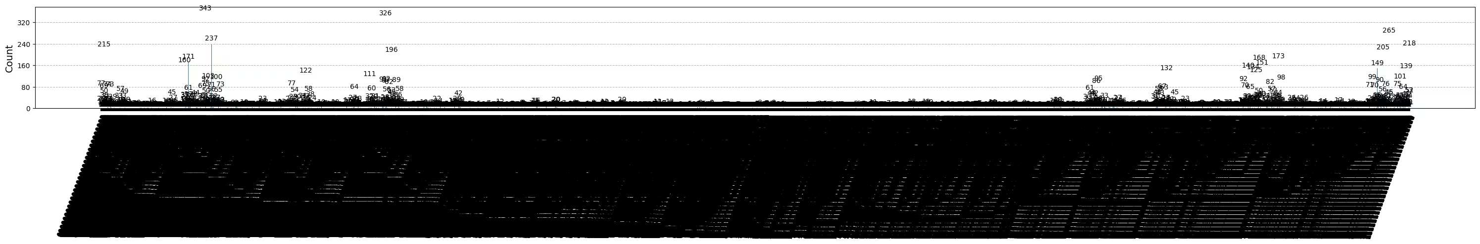
N=30: |00..0>: 4, |11..1>: 218, |3rd>: 265 (111111111111111011111111111111)
P(|00..0>)=0.0001, P(|11..1>)=0.00545
REM: Coherence (non-diagonal): 0.187073
GHZ fidelity = 0.096312 ± 0.003254
GME (genuinely multipartite entangled) test: Failed

Como você pode ver, este resultado não atendeu aos critérios.

# It will take some time
result = job_s.result()
plot_histogram(result[0].data.c.get_counts(), figsize=(30, 5))

4. Estratégia 3: Executar com as opções de supressão de erros

Você pode definir as opções de supressão de erros no Sampler V2. Consulte o guia Configurar mitigação de erros e a referência da API ExecutionOptionsV2 para mais informações.

opts = SamplerOptions()
opts.dynamical_decoupling.enable = True
opts.execution.rep_delay = 0.0005
opts.twirling.enable_gates = True

res = execute_ghz_fidelity(
    ghz_circuit=ghz3,
    physical_qubits=best_qubits,
    backend=backend,
    sampler_options=opts,
)

job_s = service.job(res[0])  # Use your job id showed above.
job_e = service.job(res[1])
print(job_s.status(), job_e.status())

DONE DONE

N = 30

# Check fidelity from job IDs
res = check_ghz_fidelity_from_jobs(
    sampler_job=job_s,
    estimator_job=job_e,
    num_qubits=N,
)

N=30: |00..0>: 1459, |11..1>: 1543, |3rd>: 359 (111111111111111111111111111110)
P(|00..0>)=0.036475, P(|11..1>)=0.038575
REM: Coherence (non-diagonal): 0.165532
GHZ fidelity = 0.120291 ± 0.003369
GME (genuinely multipartite entangled) test: Failed

# It will take some time
result = job_s.result()
plot_histogram(result[0].data.c.get_counts(), figsize=(30, 5))

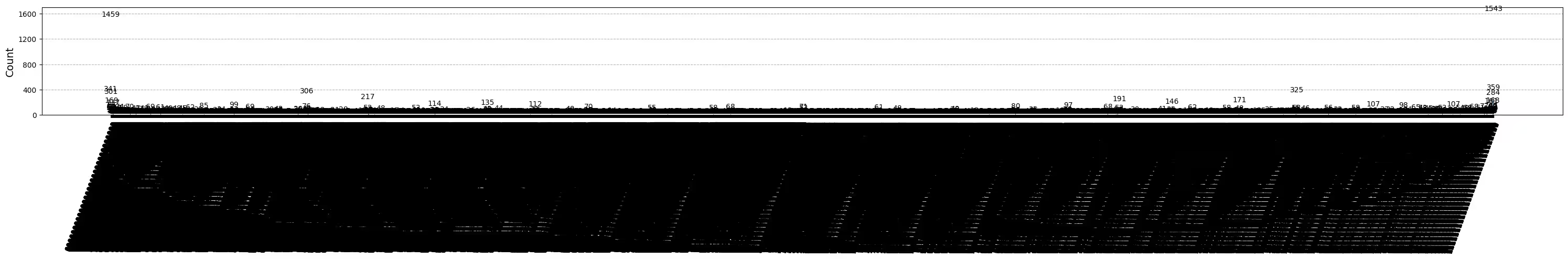
O resultado melhorou, mas ainda não atendeu aos critérios.

Vimos três ideias até agora. Você pode combiná-las e expandi-las, ou criar suas próprias ideias para construir um Circuit GHZ melhor. Agora vamos revisar o objetivo novamente.

5. Seu objetivo (recapitulação)

Construa um Circuit GHZ com 20 qubits ou mais de forma que o resultado da medição atenda aos critérios: a fidelidade do seu estado GHZ deve ser maior que 0,5.

• Você precisa usar um dispositivo Eagle (como ibm_brisbane) e definir o número de shots como 40.000.
• Você deve executar o Circuit GHZ usando a função execute_ghz_fidelity e calcular a fidelidade usando a função check_ghz_fidelity_from_jobs.

Você precisa encontrar o maior Circuit GHZ — em número de qubits — que atenda aos critérios. Escreva seu código abaixo e mostre o resultado com a função check_ghz_fidelity_from_jobs.

Agora vamos implementar o mesmo fluxo de trabalho GHZ do material anterior, mas em um dispositivo Heron. Isso lhe dará experiência com o layout e os recursos dos processadores Heron. Nenhuma nova estratégia é introduzida.

O tempo estimado de QPU para executar este próximo experimento é de 4 min 40 s.

service = QiskitRuntimeService()
backend = service.backend("ibm_kingston")
# backend = service.backend("ibm_fez")

twoq_gate = "cz"
print(f"Device {backend.name} Loaded with {backend.num_qubits} qubits")
print(f"Two Qubit Gate: {twoq_gate}")

Device ibm_kingston Loaded with 156 qubits
Two Qubit Gate: cz

BAD_READOUT_ERROR_THRESHOLD = 0.1
BAD_CZGATE_ERROR_THRESHOLD = 0.1
bad_readout_qubits = [
    q
    for q in range(backend.num_qubits)
    if backend.target["measure"][(q,)].error > BAD_READOUT_ERROR_THRESHOLD
]
bad_czgate_edges = [
    qpair
    for qpair in backend.target["cz"]
    if backend.target["cz"][qpair].error > BAD_CZGATE_ERROR_THRESHOLD
]
print("Bad readout qubits:", bad_readout_qubits)
print("Bad CZ gates:", bad_czgate_edges)

Bad readout qubits: [112, 113, 120, 131, 146]
Bad CZ gates: [(111, 112), (112, 111), (112, 113), (113, 112), (120, 121), (121, 120), (130, 131), (131, 130), (145, 146), (146, 145), (146, 147), (147, 146)]

g = backend.coupling_map.graph.copy().to_undirected()
g.remove_edges_from(
    bad_czgate_edges
)  # remove edge first (otherwise might fail with a NoEdgeBetweenNodes error)
g.remove_nodes_from(bad_readout_qubits)

qubit_color = []
for i in range(backend.num_qubits):
    if i in bad_readout_qubits:
        qubit_color.append("#000000")  # black
    else:
        qubit_color.append("#8c00ff")  # purple
line_color = []
for e in backend.target.build_coupling_map().get_edges():
    if e in bad_czgate_edges:
        line_color.append("#ffffff")  # white
    else:
        line_color.append("#888888")  # gray
plot_gate_map(
    backend,
    qubit_color=qubit_color,
    line_color=line_color,
    qubit_size=60,
    font_size=30,
    figsize=(10, 10),
)

N = 40
central = 100  # Select the center node manually
# c_degree = dict(rx.betweenness_centrality(g))
# central = max(c_degree, key=c_degree.get)
# central

class TreeEdgesRecorder(rx.visit.BFSVisitor):
    def __init__(self, N):
        self.edges = []
        self.N = N

    def tree_edge(self, edge):
        self.edges.append(edge)
        if len(self.edges) >= self.N - 1:
            raise rx.visit.StopSearch()

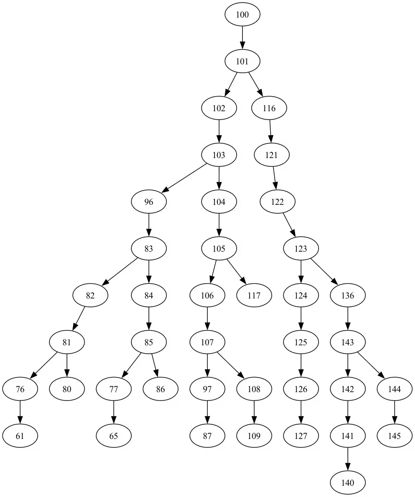
vis = TreeEdgesRecorder(N)
rx.bfs_search(g, [central], vis)
best_qubits = sorted(list(set(q for e in vis.edges for q in (e[0], e[1]))))
print("Qubits selected:", best_qubits)

Qubits selected: [61, 65, 76, 77, 80, 81, 82, 83, 84, 85, 86, 87, 96, 97, 100, 101, 102, 103, 104, 105, 106, 107, 108, 109, 116, 117, 121, 122, 123, 124, 125, 126, 127, 136, 140, 141, 142, 143, 144, 145]

qubit_color = []
for i in range(backend.num_qubits):
    if i in bad_readout_qubits:
        qubit_color.append("#000000")
    elif i in best_qubits:
        qubit_color.append("#ff00dd")
    else:
        qubit_color.append("#8c00ff")
line_color = []
for e in backend.target.build_coupling_map().get_edges():
    if e in bad_czgate_edges:
        line_color.append("#ffffff")
    else:
        line_color.append("#888888")
plot_gate_map(
    backend,
    qubit_color=qubit_color,
    line_color=line_color,
    qubit_size=60,
    font_size=30,
    figsize=(10, 10),
)

from rustworkx.visualization import graphviz_draw

tree = rx.PyDiGraph()
tree.extend_from_weighted_edge_list(vis.edges)
tree.remove_nodes_from([n for n in range(max(best_qubits) + 1) if n not in best_qubits])

graphviz_draw(tree, method="dot")

ghz_h = QuantumCircuit(max(best_qubits) + 1, N)

ghz_h.h(tree.edge_list()[0][0])  # apply H-gate to the root node
# Apply CNOT from the root node to the each edge.
for u, v in tree.edge_list():
    ghz_h.cx(u, v)
ghz_h.barrier()  # for visualization
ghz_h.measure(best_qubits, list(range(N)))
ghz_h.draw(output="mpl", idle_wires=False, fold=-1)

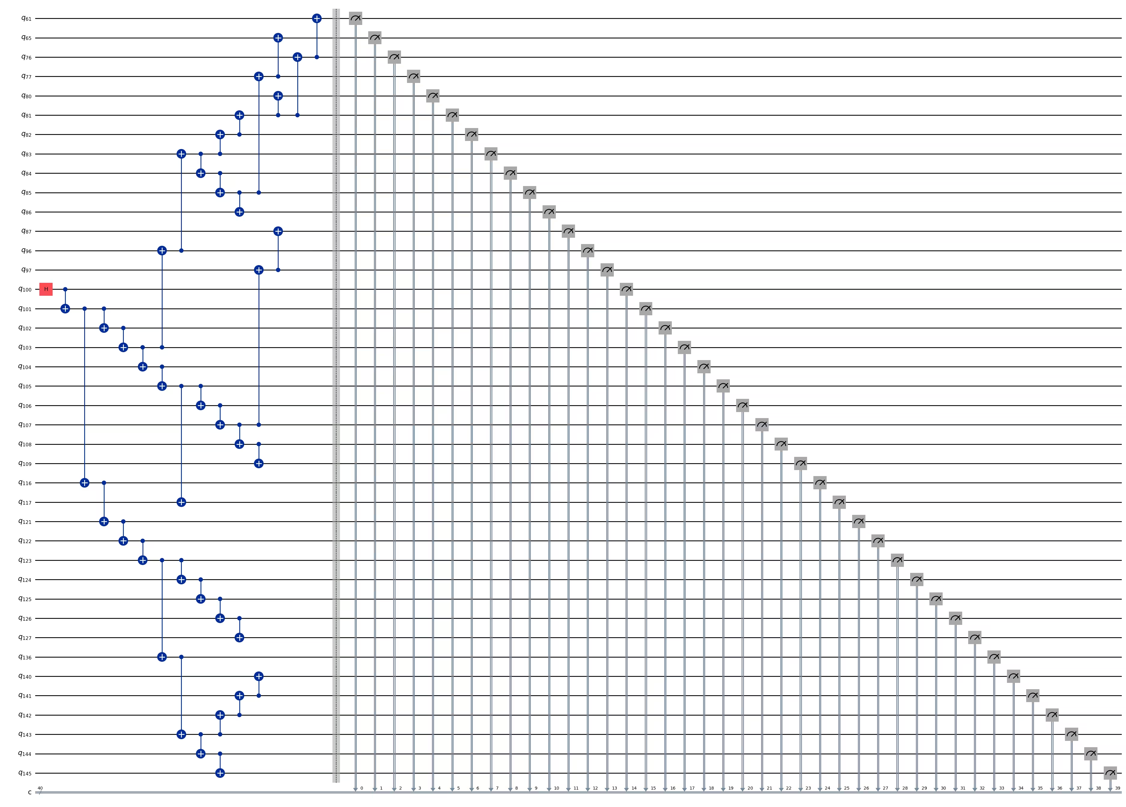
ghz_h.depth()

15

pm = generate_preset_pass_manager(1, backend=backend)
ghz_h_transpiled = pm.run(ghz_h)
ghz_h_transpiled.draw(output="mpl", idle_wires=False, fold=-1)

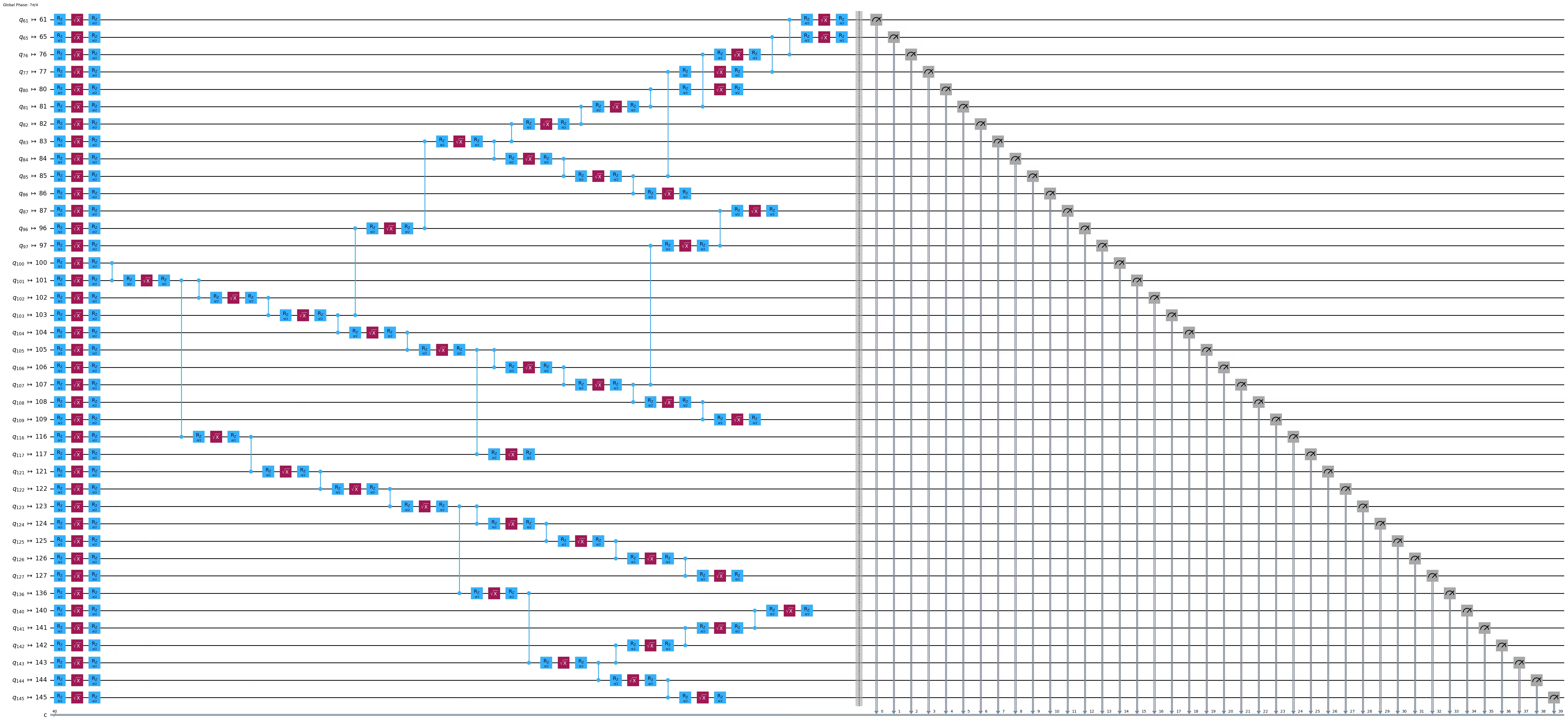
print("Depth:", ghz_h_transpiled.depth())
print(
    "Two-qubit Depth:",
    ghz_h_transpiled.depth(filter_function=lambda x: x.operation.num_qubits == 2),
)

Depth: 45
Two-qubit Depth: 13

opts = SamplerOptions()
opts.dynamical_decoupling.enable = True
opts.execution.rep_delay = 0.0005
opts.twirling.enable_gates = True

res = execute_ghz_fidelity(
    ghz_circuit=ghz_h,
    physical_qubits=best_qubits,
    backend=backend,
    sampler_options=opts,
)

job_s = service.job(res[0])  # Use your job id showed above.
job_e = service.job(res[1])
print(job_s.status(), job_e.status())

RUNNING RUNNING

# Check fidelity from job IDs
N = 40
res = check_ghz_fidelity_from_jobs(
    sampler_job=job_s,
    estimator_job=job_e,
    num_qubits=N,
)

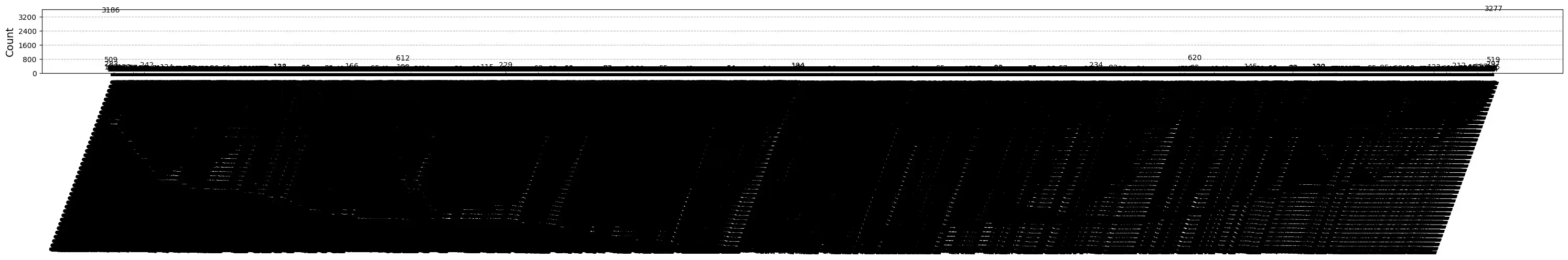
N=40: |00..0>: 3186, |11..1>: 3277, |3rd>: 620 (1111111011111111111111111111111111111111)
P(|00..0>)=0.07965, P(|11..1>)=0.081925
REM: Coherence (non-diagonal): 0.029987
GHZ fidelity = 0.095781 ± 0.002619
GME (genuinely multipartite entangled) test: Failed

# It will take some time
result = job_s.result()
plot_histogram(result[0].data.c.get_counts(), figsize=(30, 5))

Parabéns! Você concluiu sua introdução à computação quântica em escala utilitária! Agora você está preparado para fazer contribuições significativas na busca pela vantagem quântica! Obrigado por fazer do IBM Quantum® parte da sua jornada pessoal pela computação quântica.

Pesquisa pós-curso

Parabéns por concluir este curso! Por favor, reserve um momento para nos ajudar a aprimorar nosso conteúdo preenchendo esta pesquisa rápida. Seu feedback será usado para melhorar nossa oferta de conteúdo e a experiência do usuário. Obrigado!